RainbowStats Morning Note · August 25, 2026

Inflation Has Two Clocks

Labor-market pressure can start inflation moving. A different mechanism may determine whether it stays elevated.

A reduced-form RainbowStats companion to CIMEO Working Paper No. 208

Reproduce the complete analysis Open the live RainbowStats slideshow. The script, data refresh and all model panels run in the browser.

Inflation debates often compress two questions into one. What creates the initial pressure? And what allows that pressure to persist? Those questions sound similar, but they need not have the same answer.

A recent CIMEO working paper develops a structural account in which labor pressure and the pricing environment play distinct roles. Our exercise takes that intuition to the data with a deliberately simpler toolkit: a fixed-threshold regression, matched comparisons, rolling persistence, joint regressions and transfer functions.

This is not a replication of the paper's latent-state model. It is a transparent reduced-form companion built from quarterly CPI and the FRED-QD help-wanted-to-unemployed ratio, HWIURATIOX.

When the labor market crosses one

We define tightness as the logarithm of the help-wanted-to-unemployed ratio. The threshold is fixed at zero, which corresponds to a raw ratio of one: one help-wanted measure for every unemployed worker.

The split is sharp. Below or at the threshold, the estimated inflation-tightness slope is 1.367. Above it, the slope rises to 8.287. Both slopes are statistically meaningful, and the fixed-split diagnostic produces an F statistic of 6.451.

1.367Slope at or below the tightness threshold

8.287Slope above the tightness threshold

6.451Fixed-split diagnostic F statistic

RainbowStats fixed-threshold regression summary showing a much steeper inflation slope above the labor tightness threshold — Figure 1. The inflation-tightness slope becomes much steeper after HWIURATIOX rises above one. The split improves the residual sum of squares by about 4.7%.

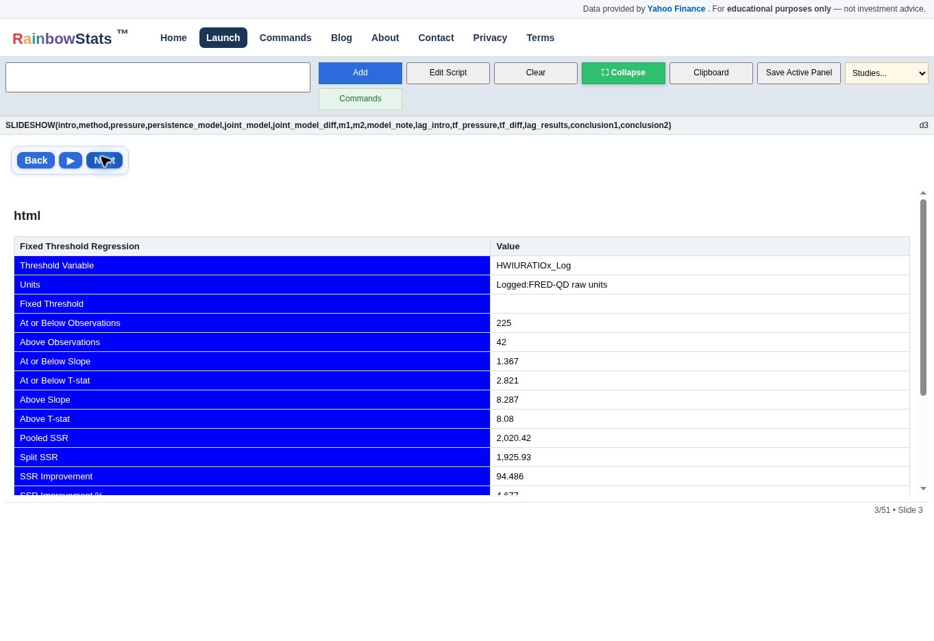
The result does not say tightness explains every inflation episode. It says the relationship is nonlinear: the same incremental movement in tightness is associated with a much larger inflation response once labor demand is already pressing against available workers.

Pressure and persistence are different variables

We estimate a rolling 20-quarter inflation-persistence coefficient, called rho. In the levels regression, tightness and persistence both help explain four-quarter inflation. Their simple linear interaction, however, is weak. That is already useful: the data do not require a mechanically multiplicative story in which tightness and persistence always reinforce each other.

Differencing changes the emphasis. Changes in tightness carry a coefficient of 1.47 with a t statistic of 3.79. Changes in persistence and in the interaction contribute little. The Durbin-Watson statistic improves from 0.174 in levels to 1.816 in differences, making the acceleration model considerably cleaner statistically.

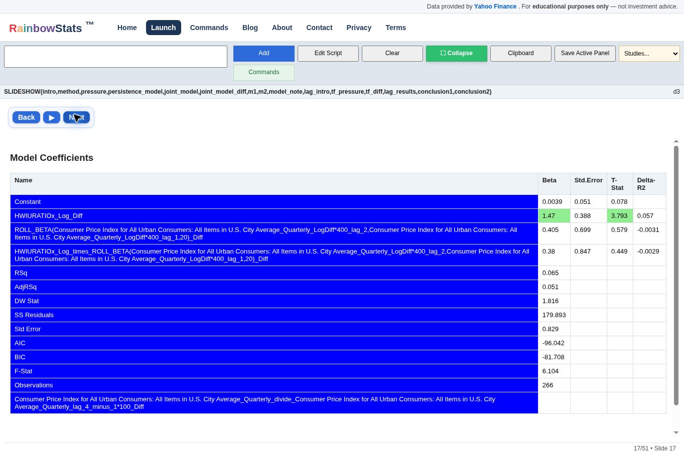
RainbowStats regression table for changes in inflation, labor tightness, persistence and their interaction — Figure 2. In the differenced model, the change in labor tightness is the clear explanatory variable. The persistence and interaction terms are small and statistically weak.

Labor pressure appears to govern movement in inflation. Persistence helps characterize the environment in which inflation remains elevated.

A matched comparison asks a different question

The threshold regression estimates a change in slope. Matching estimates a conditional difference in mean inflation. Those are not the same quantity, so the results need not be identical.

After matching high- and low-persistence observations on labor tightness, the analysis retains 88 pairs. Average inflation is 5.355% in the high-persistence group and 2.354% among matched controls: a difference of 3.001 percentage points with a paired t statistic of 7.53.

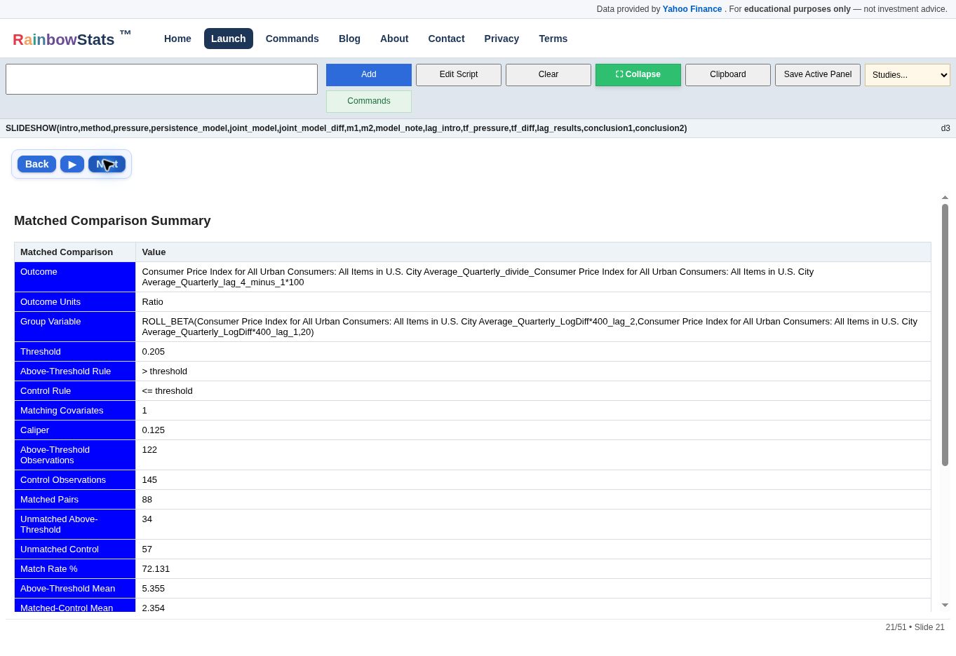
RainbowStats matched comparison summary for high- and low-persistence inflation periods after balancing labor tightness — Figure 3. High-persistence periods display materially higher inflation after matching on labor tightness. This is descriptive evidence, not a causal estimate.

The companion comparison—tight versus slack labor markets after balancing persistence—shows little matched difference in mean inflation. That does not negate the threshold result. One model asks whether the slope steepens; the other asks whether two balanced groups have different average outcomes.

The transfer function adds the clock

A contemporaneous regression can tell us that tightness and inflation move together. A transfer function asks when the movement arrives. RainbowStats first filters the input and output series, examines the cross-correlation of their innovations, and then estimates the selected current and lagged effects.

tf_pressure=TRANSFER_FUNCTION(piq,tightness)
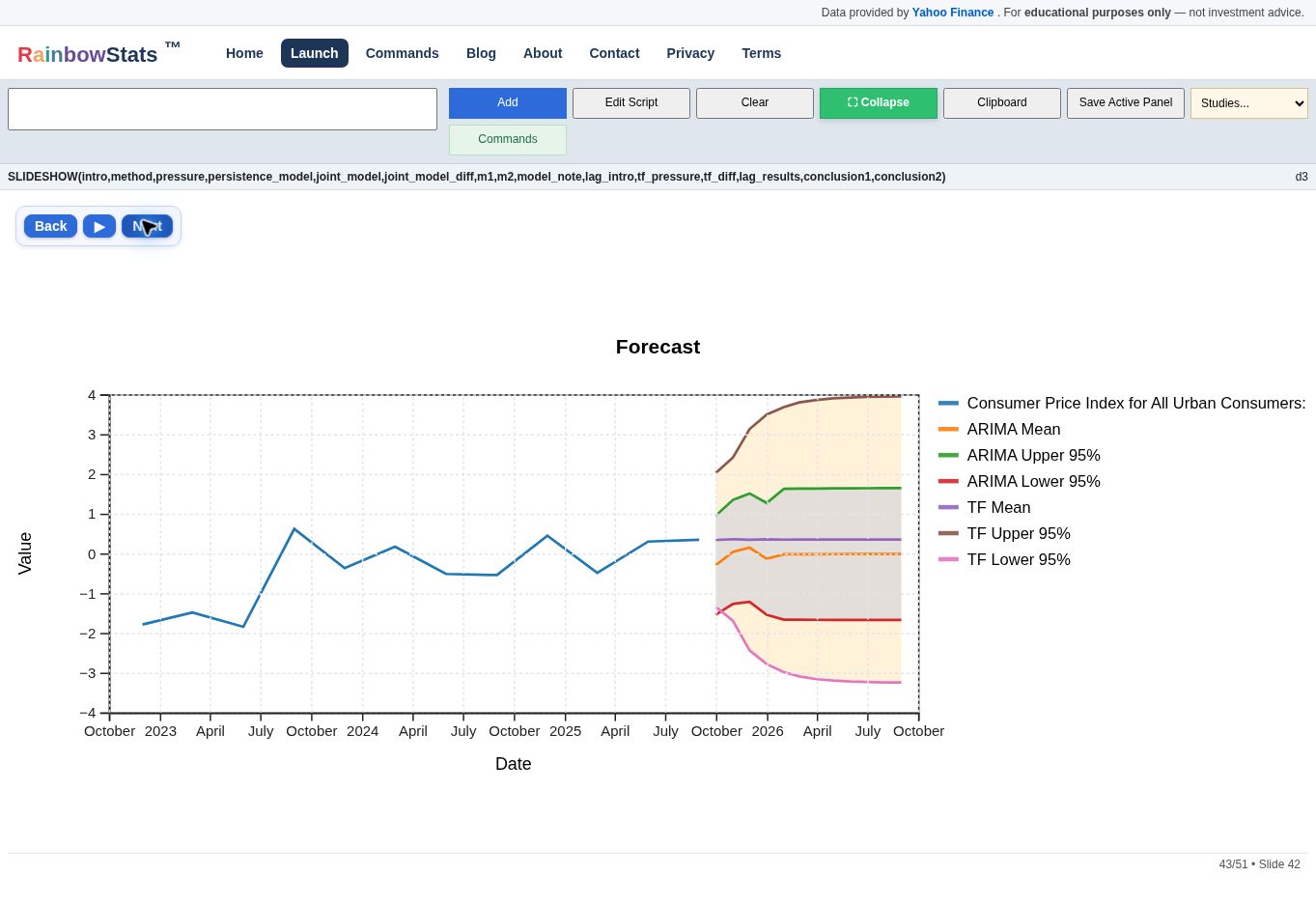
tf_diff=TRANSFER_FUNCTION(DIFF(pi4),DIFF(tightness))

The first model relates quarterly annualized inflation to the level of labor tightness. The second is the more conservative specification: it relates the change in four-quarter inflation to the change in tightness, reducing the danger that two persistent series merely drift together.

In the differenced transfer function, the strongest filtered cross-correlation occurs contemporaneously. The estimated dynamic response then has two pieces:

Filtered ΔInflation_t = 0.013 + 0.863·Filtered ΔTightness_t − 0.723·Filtered ΔTightness_t−8 + ε_t

The contemporaneous coefficient is positive, with a t statistic of 2.84. The eight-quarter coefficient is negative, with a t statistic of −2.39. Residual autocorrelation is well controlled: the Durbin-Watson statistic is 2.07.

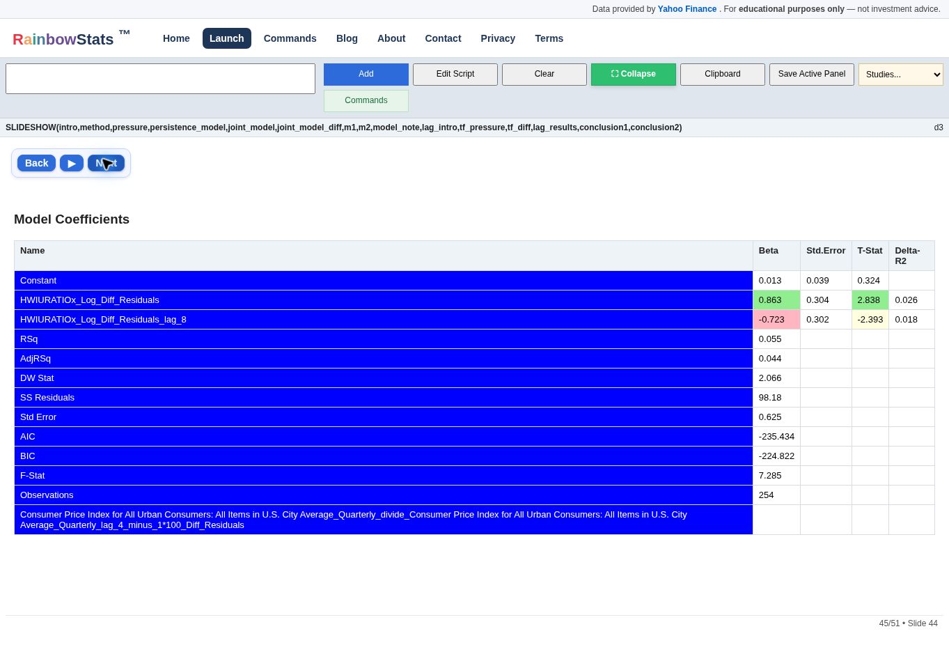
RainbowStats transfer-function coefficient table showing a positive immediate tightness effect and negative effect at eight quarters — Figure 4. The differenced transfer function finds an immediate positive response followed by a reversal near eight quarters.

That two-horizon pattern is economically intuitive. Tightening initially accelerates inflation. Roughly two years later, much of the impulse is reversed. Labor pressure can move inflation without permanently raising its path.

RainbowStats transfer-function forecast with ARIMA and transfer-function confidence bands — Figure 5. The transfer-function forecast separates the baseline ARIMA path from the path that incorporates the filtered labor-tightness input. Wide bands are a reminder that dynamic forecasts remain uncertain.

The morning takeaway

The evidence supports a layered interpretation of inflation. A tight labor market creates pressure and helps explain acceleration. Persistence describes a different dimension: whether inflation remains elevated after the initial impulse. The transfer function makes the distinction visible by attaching a clock to the response.

The most defensible conclusion is modest but useful: pressure starts the process; persistence helps determine its duration. The analysis supports the working paper's intuition, but it does not identify the paper's structural states or establish a causal mechanism.

Statistical caution. The lag selection is data-driven, the explanatory power of the transfer function is modest, and rho is constructed from inflation itself. Results should be treated as descriptive evidence and tested across alternative samples, inflation measures and lag-selection rules.