From Black–Scholes to Variance Gamma
Why characteristic functions and the FFT turn one option formula into an entire pricing engine
Black–Scholes remains the common language of option markets because it does something profound: it converts a nonlinear payoff into a replicating strategy. But the model’s greatest strength is also the source of its most visible failure. A single constant volatility produces a flat implied-volatility line, while traded options routinely display smiles and skews.
The practical response is not to discard Black–Scholes. It is to retain its no-arbitrage foundation while widening the class of risk-neutral distributions. Characteristic functions provide that bridge. The fast Fourier transform supplies the computational scale. Variance Gamma provides a compact example of how skewness and heavier tails alter prices, implied volatilities and risk-neutral probability distributions.
Run the complete script in RainbowStats
This analysis uses a one-year European option strip with the following common assumptions:
| Parameter | Value |
|---|---|
| Spot price \(S_0\) | 6,600 |
| Risk-free rate \(r\) | 3.5% |
| Dividend yield \(q\) | 2.0% |
| Maturity \(T\) | 1 year |
| Diffusion scale \(\sigma\) | 20% |
| FFT damping parameter \(\alpha\) | 1.5 |
| FFT grid size \(N\) | 4,096 |
| Frequency spacing \(\eta\) | 0.25 |
| Variance Gamma asymmetry \(\theta\) | -0.10 |
| Variance Gamma activity parameter \(\nu\) | 0.20 |
The graphs use every retained strike produced by RainbowStats’ \(\operatorname{EUROPEAN\_FFT}\) calculation. They are model outputs, not illustrative curves.
The economic core: replicate the claim
A European call has the terminal payoff
\[ C(S_T)=\max(S_T-K,0). \]
Before maturity, its value depends on the distribution of the future stock price. Black–Scholes does not begin by forecasting that distribution’s expected return. It begins with replication.
Assume the stock follows
\[ dS=(\mu-q)S\,dt+\sigma S\,dW. \]
Construct a portfolio containing the option and an offsetting stock position:
\[ \Pi=C-\Delta S, \qquad \Delta=\frac{\partial C}{\partial S}. \]
Ito’s lemma describes the option’s local change. Choosing \(\Delta\) equal to the option’s spot sensitivity cancels the random \(dW\) term. Over the instant, the hedged portfolio is locally riskless. No-arbitrage then requires it to earn the risk-free rate.
The result is the Black–Scholes partial differential equation:
\[ \frac{\partial C}{\partial t} +\frac{1}{2}\sigma^2S^2\frac{\partial^2 C}{\partial S^2} +(r-q)S\frac{\partial C}{\partial S} -rC=0. \]
The expected stock return \(\mu\) has disappeared. That is the essential economic result. The option price follows from the cost of replication, not from an investor’s forecast of the stock’s expected return.
The PDE is solved backward from
\[ C(S,T)=\max(S-K,0). \]
Equivalently, the option is the discounted risk-neutral expected payoff:
\[ C_0=e^{-rT}\mathbb{E}^{\mathbb{Q}}\!\left[\max(S_T-K,0)\right]. \]
Under the risk-neutral measure, the stock’s drift becomes its carry rate \(r-q\).
The benchmark closed form
For a European call, the familiar solution is
\[ C_0=S_0e^{-qT}\Phi(d_1)-Ke^{-rT}\Phi(d_2), \]
where
\[ d_1= \frac{\ln(S_0/K)+(r-q+\tfrac{1}{2}\sigma^2)T} {\sigma\sqrt{T}}, \qquad d_2=d_1-\sigma\sqrt{T}. \]
Black–Scholes is more than a price calculator. It converts prices into a common quoting convention—implied volatility—and generates the sensitivities used to hedge an option book:
\[ \Delta=\frac{\partial C}{\partial S}, \qquad \Gamma=\frac{\partial^2 C}{\partial S^2}, \qquad \text{Vega}=\frac{\partial C}{\partial \sigma}, \qquad \Theta=\frac{\partial C}{\partial t}, \qquad \rho=\frac{\partial C}{\partial r}. \]
A trader may reject constant volatility as a literal description of the world and still use Black–Scholes every day to quote, compare and hedge options.
Prices across the strike strip
The FFT engine prices the full option strip in one calculation. Call prices decline with the strike because the right to buy becomes less valuable as the contractual purchase price rises.
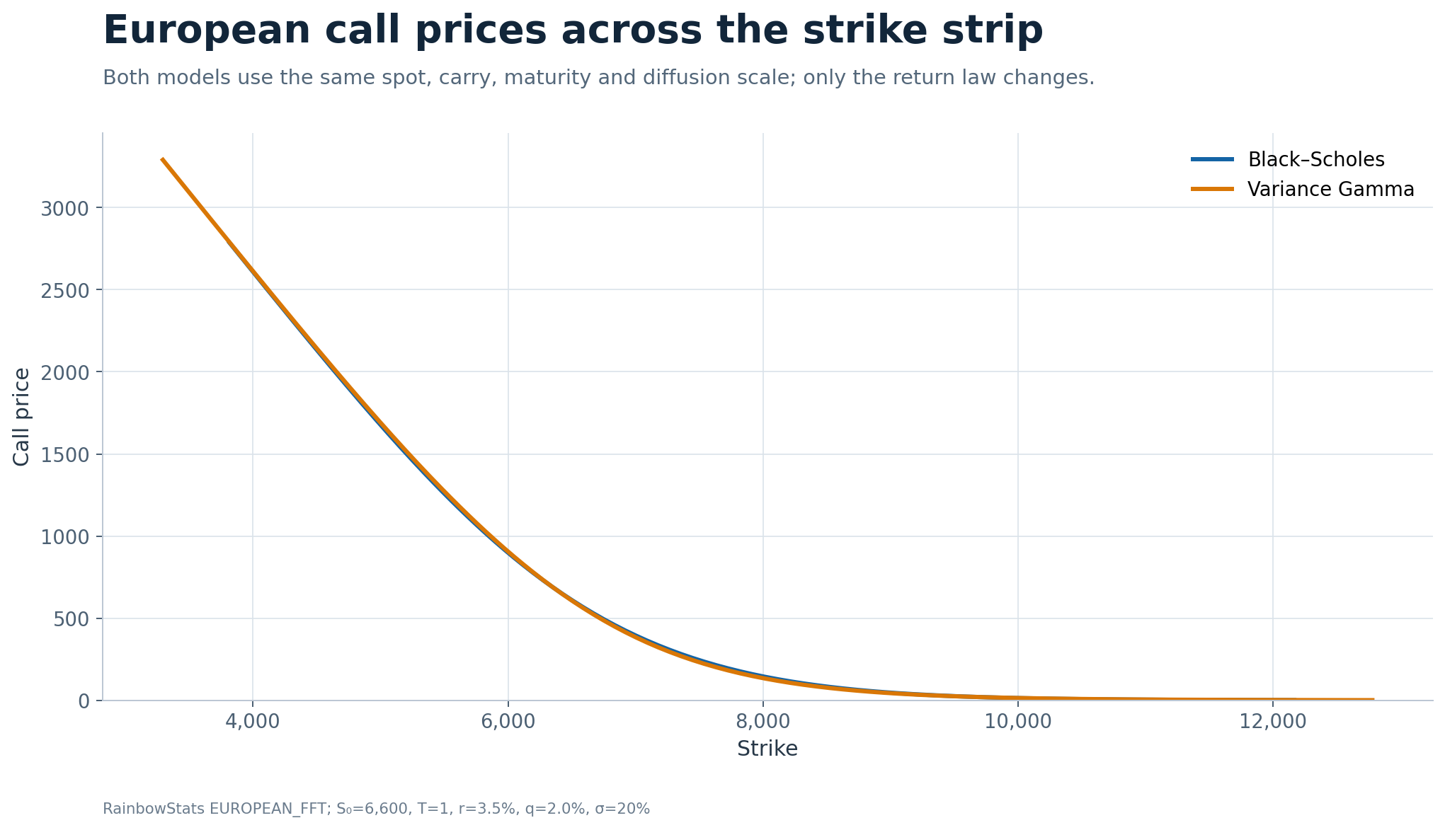
The two call-price curves appear close when plotted in levels. That is not evidence that the choice of distribution is irrelevant. The option price itself changes by only a small amount relative to a 6,600 spot price, but those changes are economically meaningful in a leveraged instrument and become conspicuous when expressed as implied volatility.
Put prices rise with the strike because a higher strike makes the right to sell more valuable.
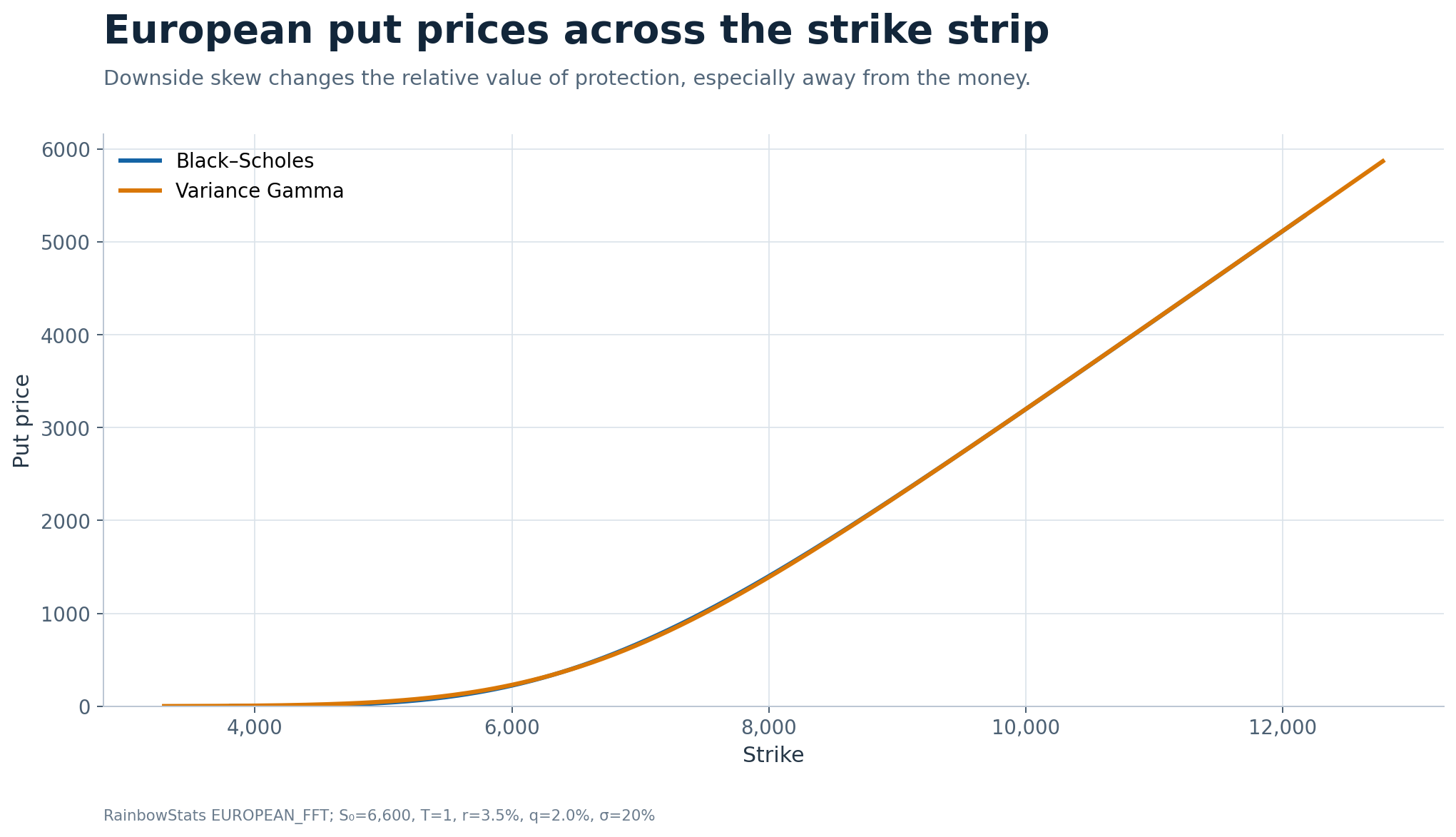
The call and put comparisons obey put–call parity. Because both models use the same spot, carry and maturity, the model-induced change in a call price equals the model-induced change in the corresponding put price. That fact becomes visible later when the two price-difference curves lie directly on top of one another.
The model’s visible failure: volatility is not flat
If constant-volatility lognormal returns were an exact description of the market, every strike for a fixed maturity would imply the same volatility:
\[ \sigma_{\text{impl}}(K,T)=\text{constant}. \]
That is precisely what the Black–Scholes benchmark produces in the graph below: a flat 20% line. The Variance Gamma prices, when translated back into Black–Scholes implied volatilities, produce a curved and asymmetric profile.
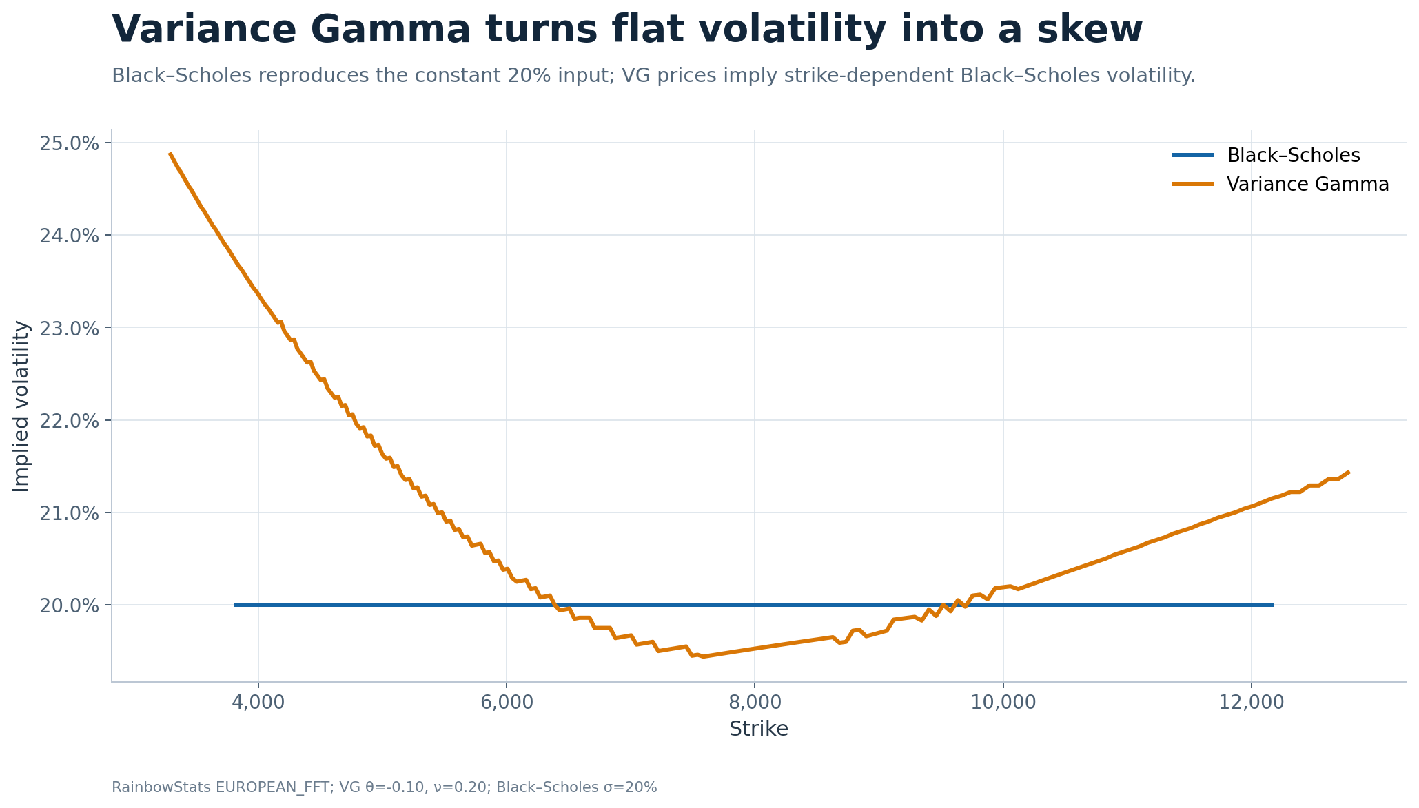
With \(\theta=-0.10\), low strikes carry substantially higher implied volatility than the Black–Scholes benchmark. Around the center of the strip, VG implied volatility falls slightly below 20%, before rising again at high strikes. At the retained strike nearest spot—approximately 6,587—the VG implied volatility is about 19.86%, compared with exactly 20% for Black–Scholes.
This is the key interpretive point: the skew is not an extra input pasted onto the price curve. It is the Black–Scholes translation of prices generated by a different risk-neutral distribution.
Characteristic functions widen the model class
Let the log return be
\[ X_T=\ln(S_T/S_0). \]
Its risk-neutral characteristic function is
\[ \varphi_T(u) = \mathbb{E}^{\mathbb{Q}}\!\left[e^{iuX_T}\right]. \]
A characteristic function uniquely determines a probability distribution. More importantly for computation, many distributions that have awkward density functions have compact characteristic functions.
For Black–Scholes log returns,
\[ \varphi_{BS}(u) = \exp\!\left[ iu\left(r-q-\frac{1}{2}\sigma^2\right)T -\frac{1}{2}\sigma^2u^2T \right]. \]
RainbowStats passes this expression directly into the FFT pricer. The entire Black–Scholes strip is generated with one equation:
BS=EUROPEAN_FFT(SYM(EXP(I*U*(R-Q-0.5*SIG^2)*T-0.5*SIG^2*U^2*T)),S0,Spot,R,Rate,Q,Dividend,T,Maturity,ALPHA,Alpha,N,4096,ETA,Eta,SIG,Volatility,CF_RETURN,1)The pricing principle has not changed. The option remains a discounted risk-neutral expectation. Only the computational representation has changed.
Fourier pricing and exponential damping
Write log strike as
\[ k=\ln K. \]
A call-price function does not decay sufficiently quickly at all ends of the strike domain for a direct Fourier transform to be convenient. The Carr–Madan construction multiplies the call price by an exponential damping factor:
\[ c_\alpha(k)=e^{\alpha k}C(k), \qquad \alpha>0. \]
Let the characteristic function of the terminal log price be
\[ \Phi_T(u) = \mathbb{E}^{\mathbb{Q}}\!\left[e^{iu\ln S_T}\right] = S_0^{iu}\varphi_T(u). \]
Define
\[ \psi(v) = \frac{ e^{-rT}\Phi_T\!\left(v-(\alpha+1)i\right) }{ \alpha^2+\alpha-v^2+i(2\alpha+1)v }. \]
The call price is recovered by Fourier inversion:
\[ C(k) = \frac{e^{-\alpha k}}{\pi} \int_0^\infty \operatorname{Re}\!\left[ e^{-ivk}\psi(v) \right]\,dv. \]
The model enters through the characteristic function. Replace \(\varphi_{BS}\) with another valid risk-neutral characteristic function and the pricing engine remains largely unchanged.
Why the FFT matters
A numerical integration performed separately for every strike repeats much of the same work. The fast Fourier transform uses the regularity of the frequency and log-strike grids to compute the complete strip together.
Sample frequencies as
\[ v_j=j\eta. \]
If the log-strike spacing is \(\lambda\), the standard FFT grid relationship is
\[ \lambda\eta=\frac{2\pi}{N}. \]
The computational cost falls from the rough scale of repeated \(N\)-point integrations to
\[ O(N\log N) \]
for the transform.
The advantages are practical:
- Speed. Thousands of strikes can be valued in a single transform.
- Consistency. Every strike uses the same model parameters and integration grid.
- Extensibility. Any model with a tractable characteristic function can enter the same pricing framework.
- Calibration. Fast strip pricing makes repeated optimization across model parameters feasible.
- Distributional output. The same transform machinery can recover densities and cumulative distributions, not merely prices.
FFT is not automatic accuracy. The damping parameter, grid size, frequency spacing, strike coverage and interpolation scheme all matter. Deep in-the-money and deep out-of-the-money prices are especially unforgiving because small absolute errors can become large relative errors.
Variance Gamma: change the clock, change the distribution
Variance Gamma evaluates Brownian motion on a random gamma clock. Let \(G_t\) be a gamma process with mean \(t\) and variance \(\nu t\). Define the VG innovation
\[ Y_t=\theta G_t+\sigma W_{G_t}. \]
The risk-neutral log return is
\[ X_t=(r-q+\omega)t+Y_t. \]
The parameters have distinct roles:
- \(\sigma\) controls the Brownian diffusion scale.
- \(\theta\) controls asymmetry.
- \(\nu\) controls the variability of the random clock and therefore affects tail thickness and jump activity.
The martingale correction is
\[ \omega= \frac{1}{\nu} \ln\!\left( 1-\theta\nu-\frac{1}{2}\sigma^2\nu \right), \]
subject to
\[ 1-\theta\nu-\frac{1}{2}\sigma^2\nu>0. \]
The risk-neutral log-return characteristic function is
\[ \varphi_{VG}(u) = e^{iu(r-q+\omega)T} \left( 1-i\theta\nu u+\frac{1}{2}\sigma^2\nu u^2 \right)^{-T/\nu}. \]
The density is more complicated than the Black–Scholes lognormal density. The characteristic function is not. That is exactly where Fourier pricing earns its keep.
The distribution behind the skew
The next graph compares the model-implied risk-neutral densities of the terminal stock price.
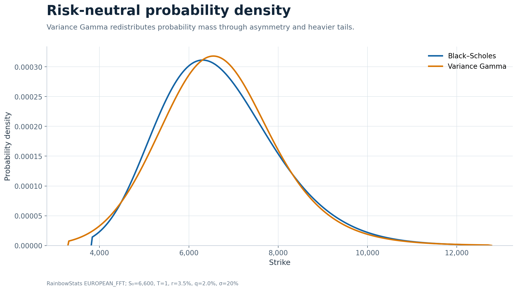
The Black–Scholes density peaks near a terminal price of 6,310 in the retained grid. The VG density peaks farther to the right, near 6,546, and is slightly more concentrated at its mode. That observation alone does not describe the tail changes. Two densities can have similar centers while assigning meaningfully different probability to the regions where option payoffs are most nonlinear.
The cumulative distribution function answers a more direct threshold question:
\[ F(K)=\mathbb{Q}(S_T\le K). \]
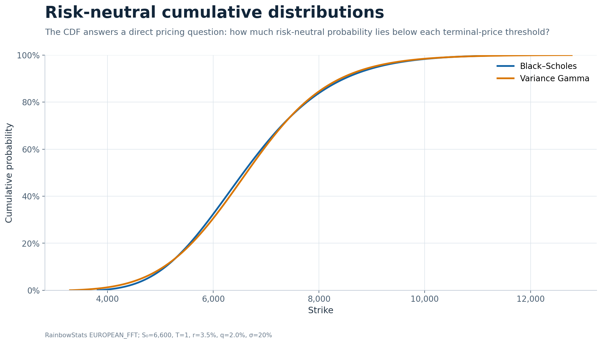
The curves are close in levels, but subtracting them reveals the structure hidden by the common 0–100% scale.
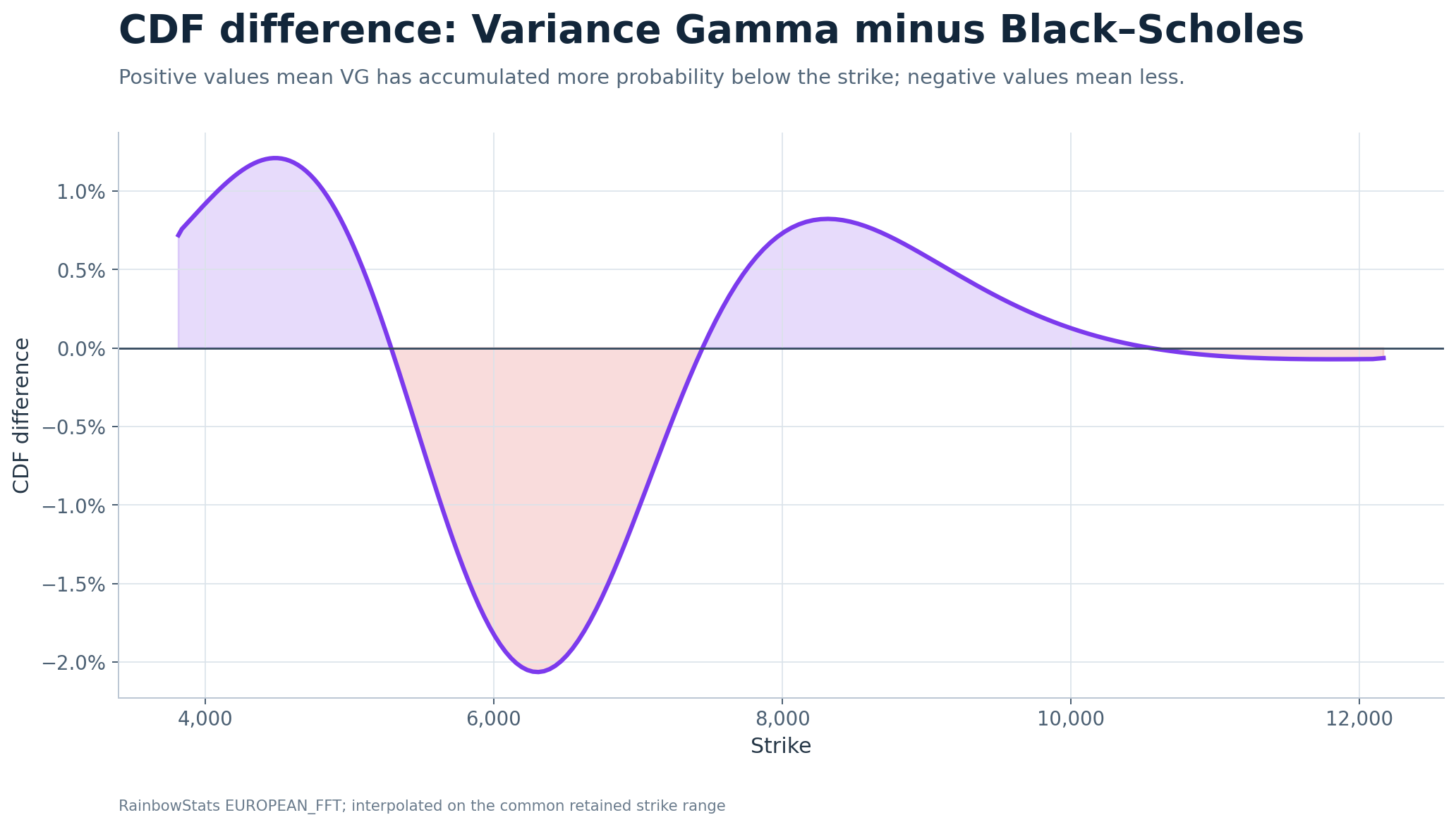
A positive difference means VG has accumulated more risk-neutral probability below that strike. A negative difference means it has accumulated less.
For this parameterization, the VG-minus-Black–Scholes CDF difference reaches approximately +1.21 percentage points near a 4,475 strike and approximately −2.06 percentage points near a 6,310 strike. The difference then becomes positive again above the central region before gradually converging toward zero in the far right tail.
This alternating pattern is more informative than the word “skew.” It shows exactly where probability mass has been added and removed relative to Black–Scholes.
Distributional differences become price differences
The same disagreement appears in option prices.
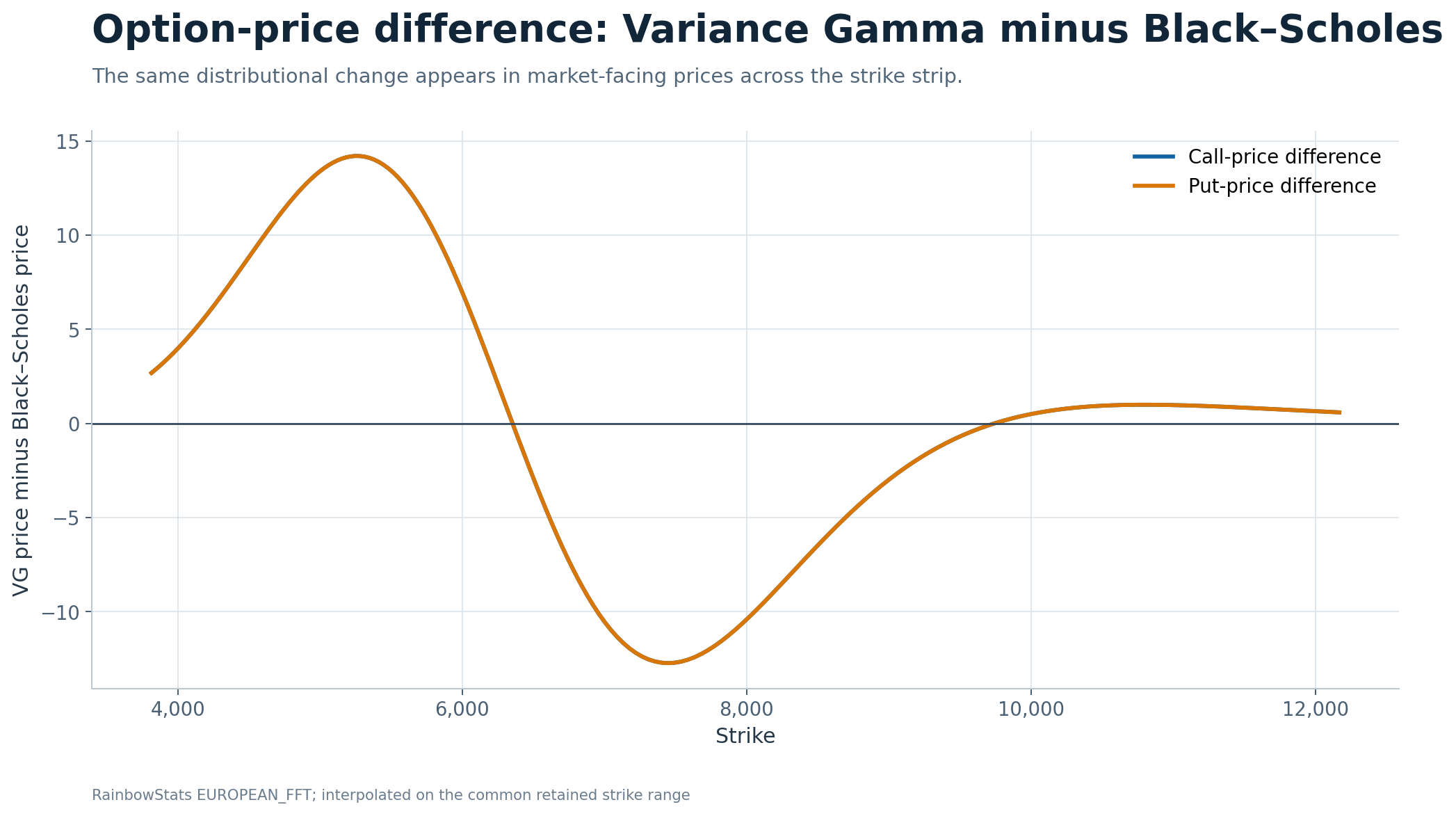
The VG-minus-Black–Scholes price difference peaks at roughly +14.20 near a 5,249 strike and reaches approximately −12.72 near a 7,446 strike over the common retained range.
The call- and put-price difference curves overlap. That is not a plotting mistake. Put–call parity implies
\[ C-P=S_0e^{-qT}-Ke^{-rT}. \]
The right-hand side is identical under both models because spot, rates, dividends and maturity are held fixed. Therefore
\[ (C_{VG}-C_{BS})-(P_{VG}-P_{BS})=0, \]
and consequently
\[ C_{VG}-C_{BS}=P_{VG}-P_{BS}. \]
The distribution changes the option’s time value, but it cannot violate a static no-arbitrage identity.
Prices, implied volatility and distributions are one story
It is tempting to treat the price curve, volatility skew and density as separate outputs. They are three representations of the same assumptions.
- The risk-neutral distribution assigns probability to future prices.
- The option payoff weights that probability nonlinearly.
- Discounted integration produces the option price.
- Black–Scholes inversion converts that price into implied volatility.
A low-strike implied volatility above 20% means that the alternative model has produced a price that Black–Scholes can match only by increasing its volatility input at that strike. The skew is therefore a compressed market convention for a richer distributional claim.
A disciplined implementation workflow
A production FFT engine should pass several tests before it is trusted:
- Recover Black–Scholes. When supplied with the Gaussian characteristic function, FFT prices and implied volatilities should reproduce the closed-form benchmark.
- Verify the martingale condition. The discounted stock price must be a martingale under the pricing measure.
- Check no-arbitrage bounds. Calls and puts must respect intrinsic value, monotonicity and convexity.
- Confirm put–call parity. Model changes should not break static replication identities.
- Test convergence. Vary \(N\), \(\eta\) and \(\alpha\); stable prices should not depend materially on arbitrary numerical settings.
- Inspect tails. Numerical truncation is often least reliable where option values are smallest and relative errors are largest.
- Validate calibration out of sample. A model that fits every quoted strike can still be unstable across maturities or dates.
The RainbowStats output includes model diagnostics, retained-row counts, implied-volatility attempts, rejected prices and density checks. Those diagnostics belong beside the charts, not behind them.
The enduring lesson
Black–Scholes supplies the economic foundation: replication, no-arbitrage and risk-neutral valuation. Characteristic functions supply a model-neutral representation of the return distribution. FFT supplies the computational scale required to price and calibrate a strip. Variance Gamma supplies a compact example of asymmetry and heavy tails.
The progression matters. One should not jump directly to a more complicated distribution and forget the replication argument that makes the price meaningful. Nor should one preserve the Black–Scholes distribution merely because its closed form is convenient.
The better approach is modular:
- preserve the no-arbitrage foundation;
- specify a defensible risk-neutral characteristic function;
- price the full strike strip efficiently;
- translate the results into prices, implied volatilities and distributions;
- and verify that every representation tells the same story.
Run and modify the complete RainbowStats analysis
The ZIP accompanying this article includes the complete RainbowStats slideshow script, the underlying FFT output used for the graphs, publication-ready PNG and SVG versions of every figure, and this article in both HTML and Markdown.
References
- Fischer Black and Myron Scholes, “The Pricing of Options and Corporate Liabilities,” Journal of Political Economy 81(3), 1973, pp. 637–654.
- Robert C. Merton, “Theory of Rational Option Pricing,” The Bell Journal of Economics and Management Science 4(1), 1973, pp. 141–183.
- Dilip B. Madan, Peter P. Carr and Eric C. Chang, “The Variance Gamma Process and Option Pricing,” European Finance Review 2(1), 1998, pp. 79–105.
- Peter Carr and Dilip B. Madan, “Option Valuation Using the Fast Fourier Transform,” Journal of Computational Finance 2(4), 1999, pp. 61–73.