When Do Bank Reserves Become Scarce?

A public-data threshold experiment inspired by Ricardo Lagos and Gastón Navarro’s Monetary Policy Operations: Theory, Evidence, and Tools for Quantitative Analysis.

RainbowStats Sunday Morning Read · Public-data empirical note

One of the pleasures of reading a good economics paper is that it gives you new questions to ask of the data. Ricardo Lagos and Gastón Navarro build a quantitative dynamic-equilibrium theory of trading in the federal funds market and use it to estimate the aggregate demand for reserves. Their structural analysis is designed to help central banks understand monetary-policy implementation in a floor system.

Our question is deliberately simpler: can the transition between abundant and increasingly scarce reserves be detected using only readily available public aggregate data?

Read the paper that inspired this analysis · Run the full RainbowStats script

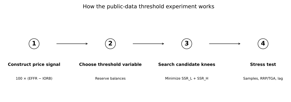
Methodology flow diagram — The experiment is intentionally transparent: construct the spread, search for the breakpoint, then try to break the result.

The empirical idea

We use the effective federal funds rate relative to the interest rate on reserve balances as the price signal:

s_t = 100 × (EFFR_t − IORB_t).

Let R_t denote reserve balances at Federal Reserve Banks. For each admissible candidate threshold R^*, RainbowStats estimates separate ordinary least-squares relationships below and above the candidate breakpoint. The selected threshold minimizes the combined residual sum of squares of the two regimes.

s_t = α_L + β_LR_t + ε_t, R_t ≤ R^*

s_t = α_H + β_HR_t + ε_t, R_t > R^*

This is not a structural replication of Lagos and Navarro. It is a reduced-form public-data test of one implication of their economics: reserve demand should become much steeper as the system approaches scarcity.

The data find a knee near $3.1 trillion

The baseline threshold regression identifies a breakpoint near $3.128 trillion of reserve balances. Below the breakpoint the estimated slope is about −0.01337 basis points per $1 billion, with a t-statistic near −3.18. Above the breakpoint the slope is economically close to flat at about +0.000158, despite a positive t-statistic in the abundant-reserve subsample.

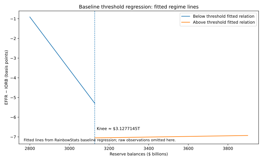
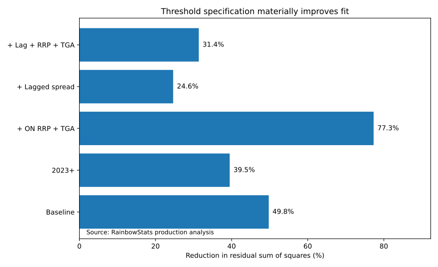
Baseline fitted reserve-demand regimes — Baseline fitted regime lines. The chart shows the fitted relationships, not the raw observations.

The two-regime model cuts residual sum of squares from about 851.1 to 427.6, an improvement of roughly 49.8%. The associated search diagnostic F-statistic is about 128. Because the breakpoint is selected by searching across candidates, we treat that F-statistic as a diagnostic rather than as a conventional fixed-break test.

Try to break the result

A useful threshold is not one that appears in a single carefully selected regression. We therefore changed the sample, added Federal Reserve balance-sheet controls, and modeled persistence in the EFFR–IORB spread.

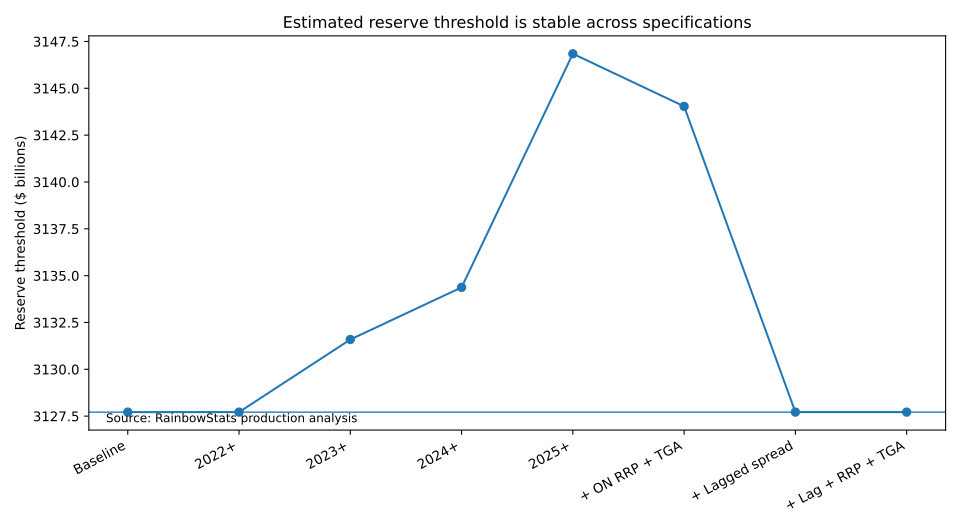
Estimated threshold across specifications — The estimated breakpoint barely moves as the sample and controls change.

Specification	Estimated threshold
Baseline	$3.128T
2022 onward	$3.128T
2023 onward	$3.132T
2024 onward	$3.134T
2025 onward	$3.147T
ON RRP + TGA controls	$3.144T
Lagged spread	$3.128T
Lagged spread + ON RRP + TGA	$3.128T

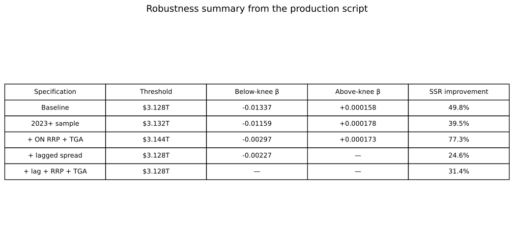
What changes substantially are the slopes. For example, after adding ON RRP and the Treasury General Account, the below-threshold reserve coefficient falls to about −0.00297. With a lagged EFFR–IORB spread it falls further to about −0.00227. That is exactly why we do not present the baseline beta as a structural causal effect.

What changes remarkably little is the location of the transition.

Regression robustness summary — Selected coefficient and fit diagnostics from the production script.

SSR improvement across specifications — The threshold model continues to improve fit under substantially different specifications.

Fed balance-sheet composition matters

Reserve balances do not move in isolation. ON RRP and the Treasury General Account are competing Federal Reserve liabilities and important liquidity channels. Once they are included, the estimated reserve slope changes materially, but the knee moves only from roughly $3.128T to $3.144T. In that conditional specification, the threshold model reduces pooled SSR by about 77.3%.

We interpret ON RRP and the TGA as robustness controls, not as exogenous instruments. The liabilities are jointly part of the operating system we are trying to understand.

Persistence matters too

The EFFR–IORB spread is strongly persistent, so a static model can attribute some of yesterday’s market conditions to today’s reserve balance. Adding a lagged spread reduces the contemporaneous reserve coefficient, but the breakpoint remains near $3.128T. Combining the lag with ON RRP and TGA leaves the threshold in essentially the same place.

The recurring result: the marginal slope is specification-sensitive; the estimated location of the nonlinear transition is far more stable.

An intriguing comparison with Lagos and Navarro

The structural paper develops a Monetary Confidence Band and reports that total reserves of about 10% of GDP would be sufficient to keep the overnight interbank rate within the target range with 99% probability on a given day. That is a different object from our reduced-form breakpoint, and the distinction should be preserved.

Yet the numerical neighborhood is striking. With nominal GDP around $32.5 trillion, our $3.128 trillion threshold is about 9.6% of GDP.

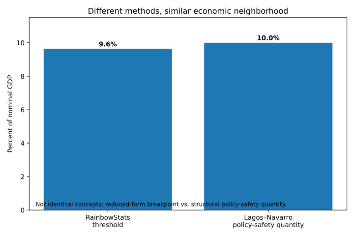
RainbowStats threshold versus Lagos Navarro policy safety quantity — Different concepts and methodologies, but a surprisingly similar economic scale.

We would not call this a replication. Lagos and Navarro use a structural model with bank heterogeneity and federal-funds-market trading; RainbowStats is performing a reduced-form threshold search in public aggregate data. The similarity is best described as independent corroborating evidence worthy of further investigation.

Why publish the script?

There is another reason for this note. The entire analysis is reproducible in RainbowStats. Reading the paper led us to add a generic THRESHOLD_REGRESSION operator, expose its results as extractable objects, and then use the same operator for sample-window, balance-sheet, and dynamic robustness exercises.

The implementation is not a one-off reproduction program. It is a reusable statistical operator that can be applied to inflation, credit, energy, labor markets, market microstructure, or any setting where a relationship may change across regimes.

Run the production analysis in RainbowStats

Conclusion

Lagos and Navarro provide the structural theory. Our exercise asks how much of the nonlinear reserve-demand story can be seen using public data and a transparent breakpoint search.

The answer is encouraging. Across changing sample windows, Federal Reserve balance-sheet controls, and a dynamic specification, U.S. money-market behavior repeatedly changes in the neighborhood of $3.1 trillion of reserve balances. At the current size of the economy, that is roughly 9–10% of GDP.

The precise marginal effect of another dollar of reserves is difficult to estimate and moves materially as the specification changes. The neighborhood in which reserves begin to matter much more appears considerably easier to detect.

A good paper gave us a testable idea. A short public-data script let us test it, challenge it, and make the entire experiment reproducible.

Reproducibility

The exact production scenario used for this article is available at the RainbowStats link above. A plain-text copy of the analysis script is also included with this HTML package as analysis_script.txt.

Sources and notes

Primary inspiration: Ricardo Lagos and Gastón Navarro, Monetary Policy Operations: Theory, Evidence, and Tools for Quantitative Analysis, forthcoming in Econometrica. The current draft describes a quantitative dynamic-equilibrium theory of fed-funds trading, global structural estimates of reserve demand, and a Monetary Confidence Band. Its approximately 10%-of-GDP figure refers to a policy-safety quantity, not to the same reduced-form breakpoint estimated here.

Public series used in the RainbowStats analysis include WRESBAL, DFF, IORB, RRPONTSYD, WTREGEN and GDP. Regression values in this article are outputs from the linked production script during the analysis session.