RainbowStats · Ecological tools

When OLS Is Not Enough

A buoy, the seasonal solar cycle, and a relationship that comes back around.

Bill Igoe · October 31, 2026

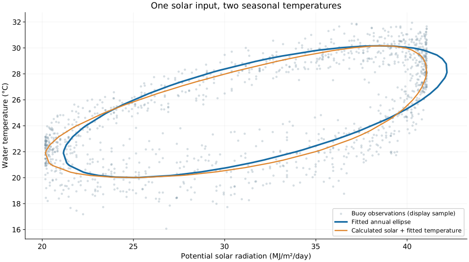
Building tools for ecological studies has a way of revealing what the next tool needs to be. We can retrieve buoy observations, locate the station with GEO_LOCATION objects, and calculate its seasonal solar environment with SOLAR. But put solar input and water temperature on a scatter plot, and a familiar straight regression line leaves something important out: the time of year.

That led us to FIT_SOLAR_ELLIPSE, a command that brings those pieces together and turns a seasonal relationship into a fitted loop.

The ocean remembers the season

Consider NOAA buoy 42040, offshore south of Dauphin Island, Alabama. Our script requests water temperatures for 2000–2025; the available paired observations in this run extend from January 1, 2000, through May 3, 2024. There are 7,631 daily pairs, with gaps in the record.

In spring, solar input is rising while the water is still relatively cool. Later in the year, the same solar input can accompany much warmer water. Heat storage, currents, mixing, and weather can all affect the response. A straight line through the scatter blends the warming and cooling parts of the year.

Here, the fitted annual water-temperature cycle follows the fitted solar cycle by about 50 days. The approximate year-bootstrap interval is 48–53 days. That timing difference gives the seasonal relationship its loop.

The command fits an annual sine-and-cosine cycle to each coordinate. When the fitted cycles are plotted against one another, their phase difference produces an ellipse. We can describe its shape, identify its foci, and follow its path through the months.

Foci of the fitted ellipse
Focus	Solar coordinate	Temperature coordinate
F₁	1.1319	1.0728
F₂	−1.1319	−1.0728

Coordinates are centered on the fitted means and scaled by the observed paired-sample standard deviations. These foci describe the geometry; they are not physical heat sources or astronomical orbital foci.

Buoy water temperature versus potential solar radiation, with observed points and two fitted seasonal loops. — The observations trace a broad seasonal loop. Blue pairs the two fitted annual harmonics; orange pairs calculated solar radiation with fitted temperature. Their difference reflects the solar series’ departure from a perfect sinusoid. This exported chart displays a sample of 1,253 observed pairs; the model uses all 7,631 pairs.

Watch a year unfold

The animation makes the timing easier to see. Follow the moving point through the months: solar input turns downward while water temperature continues to rise. The return journey follows a different path. Monthly readouts show the fitted temperature, calculated solar input, and daylight.

Animated annual solar-temperature trajectory with month labels, daylight readouts, and ellipse foci. — The native RainbowStats animated SVG, shown in standardized coordinates. Blue is the annual harmonic ellipse; orange follows calculated solar input and fitted temperature. The moving point traces the orange curve. This is a fitted reference-year cycle, rather than a replay of individual weather observations. Download the animated SVG.

A small addition with a useful purpose

The title needs one qualification: OLS still does useful work here, estimating the annual sine and cosine coefficients. What is insufficient is a single straight-line regression of temperature on solar input. The seasonal model preserves the distinction between where we are in the year and how much solar energy is potentially available.

That is the attraction of building these tools through examples. A question about buoy temperatures becomes a reusable way to examine seasonal timing in ecological data. The loop is informative—and watching it move is a pleasure.

Explore the working RainbowStats example

Appendix: reproduce and explore

Run the original script below. Its residual and SPECTRAL_ARIMA steps explore what remains after removing the fitted annual temperature harmonic; those results are outside this short introduction.

water=NDBC("42040","WTMP",2000,2025)
location=EXTRACT(NDBC_META("42040"),"geolocation")
ellipse=FIT_SOLAR_ELLIPSE(water,location)
residuals=EXTRACT(ellipse,"residuals")
additionalCycles=SPECTRAL_ARIMA(residuals)
slide(ellipse,additionalCycles)
ex(ellipse,scatter)
ex(ellipse,animation)

Interpretation. Solar radiation is calculated potential extraterrestrial energy, not measured sunlight at the sea surface. The fit describes the annual cycle; it does not isolate a causal effect, establish a physical transport time, or validate a forecast. The first-harmonic temperature fit has an in-sample R² of 0.906 and RMSE of 1.16°C. Trend, higher harmonics, and changing seasonal behavior remain outside this fit.

Uncertainty. The delay interval uses 199 whole-calendar-year bootstrap replicates, with 20 well-covered years in the record. It assumes exchangeable years; trends or dependence between years can undermine the interval. Focal-coordinate uncertainty is not estimated.

Data and method. NOAA NDBC station 42040 history; RainbowStats command reference. For related annual-cycle gain and lag concepts, see Stine and Huybers (2012), Changes in the Seasonal Cycle of Temperature and Atmospheric Circulation. This example is not a replication of that study.