When Economic Relationships Change
A mathematical paper piqued my interest. Could its ideas help us understand changes in monetary policy?
I recently came across a 2025 paper, Geometric Jensen-Shannon Divergence Between Gaussian Measures On Hilbert Space. The title is formidable, but the idea interested me: instead of comparing only averages or regression coefficients, why not compare entire probability distributions?
With ChatGPT's assistance, I added a GEOMETRIC_JS command to RainbowStats, implementing a finite-dimensional Gaussian version of the idea. Then I tried it on two familiar economic series: the unemployment rate and the federal funds rate.
Two series, two monetary-policy environments
I compared 2000–2007 with 2010–2019. The first period preceded the global financial crisis; the second covered the post-crisis recovery and the long period of exceptionally low interest rates.
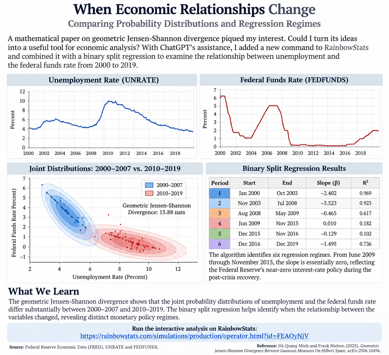
The geometric Jensen–Shannon divergence between the fitted joint distributions was approximately 15.88 nats. That is a measure of distributional difference—not a probability, percentage, or automatic significance test.
The shaded contours make the result easier to understand. Their positions show where observations concentrate; their shapes and tilts reflect variation and correlation. The two periods look different, not just in their averages but in their joint behavior.
When did the relationship change?
That led to another question. Rather than choosing a crisis date ourselves, could we let a regression algorithm search for changes over the full 2000–2019 sample?
RainbowStats' BINARY_SPLIT command identified six regression regimes when explaining the federal funds rate using unemployment:
| Period | Slope | R² |
|---|---|---|
| Jan 2000–Oct 2003 | −2.402 | 0.969 |
| Nov 2003–Jul 2008 | −3.523 | 0.923 |
| Aug 2008–May 2009 | −0.465 | 0.617 |
| Jun 2009–Nov 2015 | +0.010 | 0.182 |
| Dec 2015–Nov 2016 | −0.129 | 0.102 |
| Dec 2016–Dec 2019 | −1.495 | 0.736 |
The striking result is June 2009 through November 2015. Unemployment declined considerably, yet the federal funds rate barely moved. The estimated slope was essentially zero—consistent with the Federal Reserve maintaining near-zero policy rates during the recovery.
By 2016–2019, a more pronounced negative relationship had reappeared as policy normalized.
Two methods, one story
Geometric Jensen–Shannon divergence asks how different the joint probability distributions are. Binary split regression asks when the estimated relationship changes. Together they provide a more informative picture than either method alone.
Neither establishes causation. The Gaussian comparison depends on modeling assumptions, and the algorithm-selected breakpoints are descriptive until subjected to formal structural-break testing. Still, they offer a useful way to explore economic history.
Four lines become another question
I am retired, and I enjoy following questions that catch my attention, often while riding my bicycle. This time, a mathematical paper led to a new RainbowStats command, an attractive probability contour chart, and a second experiment with a method already available on the site.
That's what makes this enjoyable. One question leads to another.
Reproduce the analysis
P=LIST(SERIES_BETWEEN(UNRATE,20000101,20071231),SERIES_BETWEEN(FEDFUNDS,20000101,20071231))
Q=LIST(SERIES_BETWEEN(UNRATE,20100101,20191231),SERIES_BETWEEN(FEDFUNDS,20100101,20191231))
M=GEOMETRIC_JS(P,Q)
Unemployment=SERIES_BETWEEN(UNRATE,20000101,20191231)
FedFunds=SERIES_BETWEEN(FEDFUNDS,20000101,20191231)
Breaks=BINARY_SPLIT(FedFunds,Unemployment)
SLIDE(M,Breaks)