Why Central Bankers Should Be Derivative Traders
And why political policymakers need to understand the same nonlinear risks
A country can look stable while its capacity to absorb the next shock is quietly shrinking. Its bonds trade calmly. Its currency moves within a familiar range. Debt auctions continue to clear. Political leaders interpret these observations as reassurance, and central bankers interpret them as evidence that their policy framework is working. Sometimes both judgments are reasonable. Sometimes the stability depends on a combination of institutions, market expectations and interventions that will become harder to sustain as conditions change.
The difficulty is that a national balance sheet does not behave like a straight line. Adding ten percentage points to debt relative to GDP need not have the same consequences at every starting position. Nor does an increase in uncertainty have the same effect on a lightly burdened borrower and one operating with little room for disappointment. A policy can change both the expected path of repayment capacity and the range of possible outcomes around that path. These are the kinds of distinctions derivatives traders must make every day.
This essay uses a simplified Merton model and a RainbowStats comparison of thirteen countries to explore those distinctions. It asks what central bankers and political policymakers might learn from thinking about contingent claims, volatility and the distribution of losses. The purpose is to make their decisions more thoughtful. A national economy is not a trading book, but it contains exposures that can be misunderstood when policymakers concentrate on a single reassuring price.
1. The trader's question: what happens when conditions change?
A derivatives trader cannot evaluate a position solely by its current price. The trader must consider how it responds to changes in the underlying asset, volatility, funding costs and time. A position that earns small amounts repeatedly may contain a much larger loss in an unfavorable state. A hedge that works under ordinary conditions may become difficult to maintain when liquidity disappears or relationships between markets change. The relevant question is how the entire position behaves across plausible outcomes.
Policymakers face an analogous problem. A government may issue debt to build productive infrastructure, stabilize employment or support households through a temporary shock. Those choices can improve the economy's future resources. Other commitments may increase liabilities without generating comparable repayment capacity. Even when the central projection looks affordable, the uncertainty surrounding growth, revenues, financing and political implementation matters. The same expected budget outcome can be associated with very different vulnerability to adverse events.
This is why the title should be understood as an argument about habits of thought. Central bankers should examine exposures, dependencies and asymmetric outcomes with the care a good derivatives trader applies to a position. Political policymakers should ask the same questions before creating commitments. Public objectives include employment, resilience and distribution, which no trading profit can adequately represent. The trader's contribution is a disciplined way to examine the financial consequences of pursuing those objectives under uncertainty.
2. Merton's insight: debt is a claim with an asymmetric payoff
Robert C. Merton's 1974 paper, On the Pricing of Corporate Debt: The Risk Structure of Interest Rates, connects corporate liabilities with option pricing. In the simplest case, a firm has assets worth A and promises a debt payment D at maturity T. Equity receives the residual if assets exceed the obligation; creditors receive the lesser of assets and promised repayment. These payoff relationships provide the starting point for structural credit pricing.1
For our illustration, asset value follows a constant-volatility lognormal process. Under risk-neutral valuation, the drift is the constant risk-free rate r. The volatility parameter is σA, and Φ denotes the standard normal cumulative distribution function. The resulting equations give equity value E, risky debt value B, and a continuously compounded model credit spread s.
The model's risk-neutral probability of assets falling below the debt payment at maturity is Φ(−d2). This is a valuation quantity under the model's assumptions. It is not automatically the probability of an actual sovereign default. Estimating a real-world probability would require a different treatment of expected asset growth, together with evidence about the sovereign's resources, obligations and behavior. Our slideshow therefore presents a mechanism and a set of scenarios, rather than an estimated national default forecast.
The useful intuition is the asymmetry of the creditor's position. A very favorable asset outcome does not entitle the creditor to unlimited additional repayment, while an unfavorable outcome can reduce what is received. As the distribution of future assets overlaps more substantially with the repayment obligation, valuation becomes increasingly sensitive to changes in leverage and uncertainty. The equations provide a disciplined illustration of why equal increments in debt need not produce equal increments in risk.
3. A country requires a different balance-sheet interpretation
Applying this framework to a sovereign requires judgment. Countries have taxation powers, public assets, legal obligations and political choices that do not fit neatly into a corporate liquidation model. Governments issuing their own currency also have monetary institutions that can affect the form of adjustment. A nation can meet nominal obligations while households experience losses through inflation or exchange-rate changes. A corporate-style default boundary captures only part of that broader problem.
This is not a novel direction for the literature. Dale Gray, Robert Merton and Zvi Bodie's 2007 work develops a contingent-claims approach to sovereign credit risk, including risks transmitted from other sectors. Related IMF research constructs sovereign balance sheets to derive forward-looking indicators. These studies motivate the broader approach; our operator is much simpler and should not be mistaken for a calibrated implementation of their frameworks.23
GDP creates a particular interpretive challenge. It measures economic activity over a period, whereas asset value is a stock representing resources available across time. Treating one year's GDP as the sovereign's asset value would confuse these concepts. We instead scale the hypothetical fiscal asset value to GDP and state that multiplier openly. This permits comparisons on a familiar debt/GDP axis while preserving the distinction between observed economic activity and assumed repayment capacity.
In the baseline scenario, fiscal asset value is three times annual GDP. Asset volatility is 15 percent, the effective horizon is ten years, and the assumed risk-free rate is 3 percent. Total debt/GDP is represented by a single maturity obligation. Real sovereign debt has many maturities, currencies and instruments. These simplifying assumptions make the mechanism visible, while also identifying precisely what additional work would be necessary before using the model for national risk measurement.
4. The extraordinary chart—and what 100 percent means
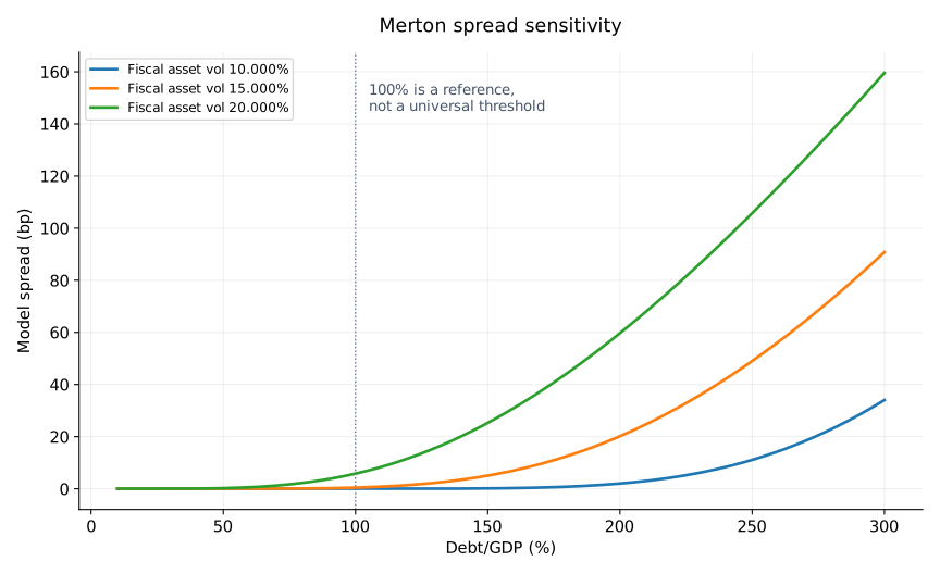
The sensitivity chart is the visual center of this exercise. At low debt ratios, model spreads lie close to zero. As debt rises, the curves move upward and become much steeper over the plotted range. Higher assumed fiscal-asset volatility raises the spread at a given debt ratio. The high-volatility curve begins showing a visible increase around the vicinity of 100 percent debt/GDP, making that region a natural place for a reader's attention to settle.
But the equations contain no special switch at 100 percent. Risk exists below that ratio, and crossing it does not automatically create a crisis. The apparent bend depends on the asset/GDP multiplier, volatility, horizon and risk-free rate, as well as the scale of the graph. A country with greater fiscal capacity or a different liability structure would occupy a different position. The number is a reference point in this particular scenario, not a universal fiscal speed limit.
| Debt/GDP (%) | Asset vol 10% | Asset vol 15% | Asset vol 20% |
|---|---|---|---|
| 50 | 0.000 | 0.001 | 0.213 |
| 100 | 0.001 | 0.427 | 5.800 |
| 150 | 0.118 | 5.028 | 25.281 |
| 200 | 1.995 | 20.156 | 59.705 |
| 250 | 11.094 | 49.024 | 105.749 |
| 300 | 34.032 | 90.804 | 159.590 |
The numerical values clarify what the eye sees. At 100 percent debt/GDP, the baseline 15 percent volatility scenario produces a spread of approximately 0.43 basis points. At 200 percent it produces approximately 20.16 basis points, and at 300 percent approximately 90.80. Under 20 percent volatility, the corresponding values are approximately 5.80, 59.71 and 159.59 basis points. The nonlinear change is substantial, but the modeled spread at 100 percent is still small under these assumptions.
The distinction strengthens the policy argument. A responsible analysis should resist replacing a flexible assessment of repayment capacity with a single politically convenient threshold. What matters is the relationship between obligations and resources across possible outcomes. A ratio that appears comfortable under one set of assumptions can look much less comfortable under another. The task is to understand the sensitivity before markets force an abrupt reassessment of the assumptions.
5. Political decisions can change both capacity and uncertainty
Political policymakers usually discuss debt in terms of spending, taxation and the deficit. The Merton perspective adds another question: what does the decision do to the distribution of future repayment capacity? Consider two hypothetical governments beginning with the same debt ratio. One borrows for a project with credible execution, durable economic benefits and transparent financing. The other creates an equally sized obligation whose implementation, costs and political durability are much less certain. Equal initial debt increases do not imply equal subsequent risk.
The project with better outcomes may support a larger fiscal resource base. The more uncertain project may widen the range of possible revenue and expenditure outcomes. Neither proposition establishes the merits of any specific policy; both are questions that a financing analysis should ask. The relevant distinction is between the size of a commitment and the economy's ability to support it under favorable and unfavorable circumstances. A headline deficit number cannot summarize both.
Political uncertainty can also arise when commitments are conditional. A guarantee looks inexpensive before it is called. Support for a financial institution may become costly at the same time tax revenues are weakening. An emergency commitment may coincide with other unexpected expenses. These are hypothetical examples of exposures whose costs depend on the state of the economy. Counting each promise separately can miss the consequences of several becoming expensive together.
The practical request to political leaders is therefore quite concrete. Explain the commitment, the resources expected to support it, the unfavorable outcomes that could undermine those resources, and who would bear the resulting losses. That discussion should include the risks of failing to act. Avoiding useful investment or withdrawing stabilization prematurely can also damage repayment capacity. A thoughtful contingent-claims perspective compares alternative distributions of outcomes rather than mechanically favoring the smallest immediate expenditure.
6. What we measured across thirteen countries
The empirical portion covers the United States, Italy, France, Greece, Spain, Germany, Japan, Canada, Switzerland, Ireland, the Netherlands, Denmark and Australia. Our principal snapshot is 2023, with historical comparisons beginning in 2000 where matching data are available. Annual general-government gross debt/GDP comes from the IMF's GGXWDG_NGDP indicator, distributed through a dated JSON snapshot on the RainbowStats server. The file contains all thirteen countries and keeps the same debt definition across the main comparisons.
This consistency matters. Our first version used World Bank central-government debt series available through FRED. Several countries lacked recent observations, leaving only six countries in the 2023 debt comparison. General government and central government are different measures, so filling individual gaps with another definition would have weakened comparability. The revised operator uses IMF general-government debt throughout the main analysis and retains a separate table showing the central-government figures where available.
Ten-year yields are monthly OECD-related series distributed through FRED. We transform them with US_ZERO to create synthetic ten-year zero prices. Bond volatility is the sample standard deviation of monthly log price changes, annualized by multiplying by the square root of twelve. These are changes in a constant-tenor synthetic price calculated from monthly yields, not returns on a purchased bond held through time. They do not measure daily bond volatility.
Currencies are quoted consistently as US dollars per unit of local currency. Higher values indicate appreciation against the dollar. Actual daily FX log changes produce annualized volatility using the square root of 252, with coverage requirements to reject inadequate years. We do not interpolate monthly bond data into invented daily observations. Annual currency appreciation compares December endpoints. Shared euro observations are not treated as independent currencies, and the dollar base is excluded from the FX cross-sections.
7. The common-currency result deserves attention
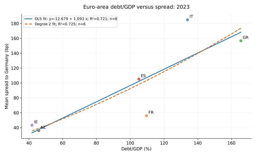
For six euro-area borrowers other than Germany, the 2023 regression relates debt/GDP to the mean ten-year yield spread over Germany. The fitted equation is:
Here the spread is measured in basis points and debt/GDP in percentage points. The slope is approximately 1.093 basis points per additional percentage point of debt/GDP. Across this small sample, higher debt ratios generally accompany wider spreads. Sharing a currency makes this a more focused comparison than one involving yields expressed in different currencies. Germany supplies the benchmark; it is not included as a forced zero-spread observation in the fitted sample.
The fit is interesting, but six observations cannot establish a general law. Countries also differ in liquidity, institutional credibility, maturity structure, growth prospects and the composition of their obligations. German yields are a market benchmark, not a direct observation of a pure risk-free rate. The measured spread can contain several premiums.
The model spreads also differ markedly from observed spreads. Under our shared assumptions, Italy's model spread is about 2.68 basis points, compared with an observed German-relative spread of about 184.87. Greece's corresponding figures are approximately 8.35 and 156.71. The mismatch shows why these scenarios are not country-specific forecasts.
8. The broader sample overturns an easy story
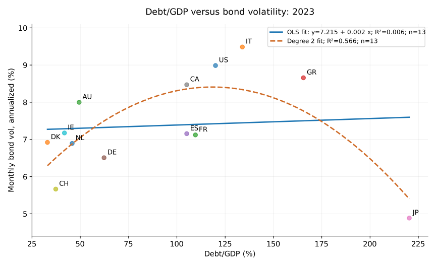
Across all thirteen countries, the 2023 regression of bond volatility on debt/GDP has an R² of only 0.006. The straight line explains almost none of the observed cross-country variation in this measure of bond volatility.
Because Merton is nonlinear, we also merge a degree-2 polynomial fit onto each debt/GDP scatter, keeping the linear fit visible and using exactly the same observations. In the thirteen-country snapshot, quadratic R² rises to 0.566; adjusted R² is 0.480, compared with −0.085 for the straight line. The fitted curve is approximately y = 4.34458 + 0.0686415 x − 0.000289823 x², with debt/GDP in percentage points. It reaches its maximum near 118% and then falls. Japan occupies the high-debt, low-volatility end of the sample. This is a descriptive inverted-U relationship, not confirmation of a convex increase in sovereign credit risk beyond 100% debt/GDP. A flexible fit can persuade us that a straight line misses structure without persuading us of the wrong economic mechanism.
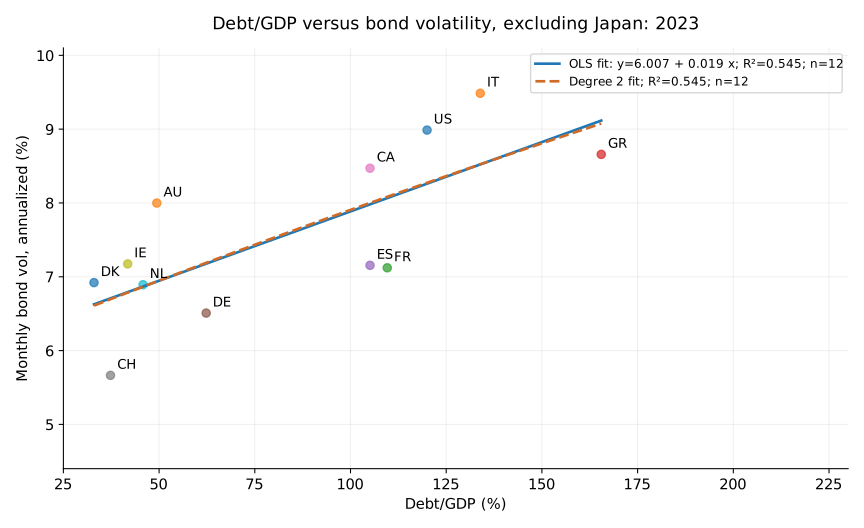
Keep both charts. Excluding Japan gives twelve observations: the linear fit is y = 6.007 + 0.018783 x, with R² = 0.545 and adjusted R² = 0.500. Quadratic R² is 0.545, with adjusted R² = 0.444. Japan strongly shapes the full-sample curvature; without it, the relationship is broadly increasing and almost linear. This is a sensitivity check. BOJ purchases and yield-curve control are documented policy interventions, not conjecture. The remaining question is how much those interventions explain Japan's unusual position; the scatter does not quantify that contribution.
Adding a squared term always preserves or increases ordinary in-sample R². That is why both lines and adjusted R² belong in the comparison. For the six euro-area borrowers, quadratic R² is 0.725 versus linear R² of 0.721, while adjusted R² falls from 0.652 to 0.542. Here the extra curvature contributes little. In the five-country currency-appreciation comparison, R² rises only from 0.662 to 0.667 and adjusted R² falls from 0.549 to 0.333. These small samples cannot reliably locate a policy threshold. The polynomial is an empirical approximation over the observed range, not the Merton equation itself, and it should not be extrapolated into unobserved debt regimes.
The historical pooled comparison also has a weak fit: Linear and quadratic R² both round to 0.029 across 310 matched country-year observations; adjusted R² falls from 0.026 to 0.023 with the extra term. Repeated observations from the same countries are not independent experiments, and the pooled line does not control for country characteristics or common global shocks. It nevertheless provides a useful descriptive check. The simple proposition that more sovereign debt reliably produces greater observed bond volatility is not supported by these particular regressions.
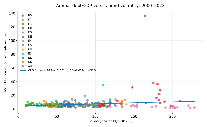
A derivatives perspective helps explain why this is not fatal to the exercise. Bond prices respond to interest rates, term premiums, liquidity and policy regimes as well as credit concerns. The Merton curves vary hypothetical asset uncertainty while holding other assumptions fixed. Our empirical bond volatility measures a different object in an environment where those other conditions change. Expecting a simple debt ratio to reproduce the theoretical curve would confuse an observed outcome with a model input.
The BOJ deliberately constrained Japanese government-bond yields through yield-curve control and bond purchases. My interpretation is that this intervention helps explain the downward bend: observed volatility is partly a policy outcome. Japan's high-debt, low-volatility position is consistent with that hypothesis, and the later rise in both bond and FX volatility makes its policy transition worth studying. Suppressed market volatility need not mean underlying fiscal uncertainty has disappeared. The scatter cannot identify how much calm comes from intervention rather than investor composition, domestic savings, inflation expectations or other institutions. Establishing suppression requires evidence on purchases, policy constraints and credible comparison periods. This is the argument to investigate, not a causal estimate already delivered by the quadratic.
9. Currency movements add information, with a small-sample warning
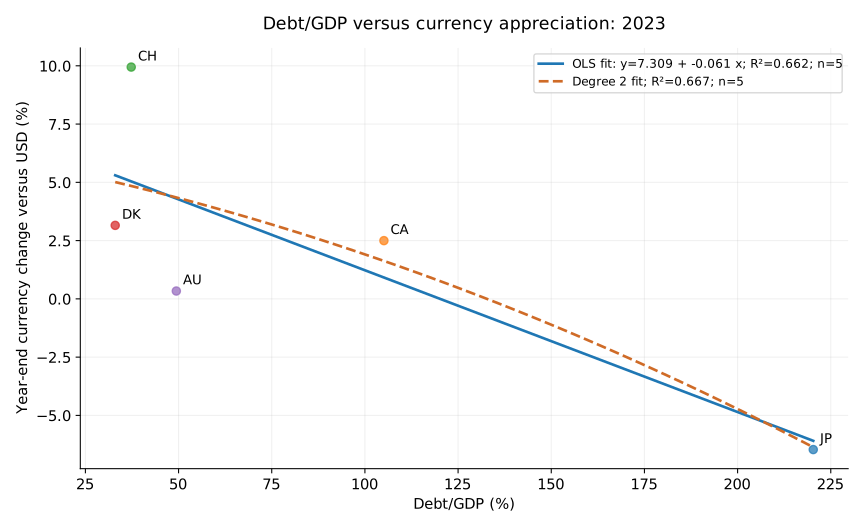
The 2023 cross-section for the five non-euro, non-dollar currencies relates annual appreciation to their countries' debt ratios. Its fitted relationship has R² of 0.662, with a slope of approximately −0.061 percentage points of appreciation per percentage point of debt/GDP. Japan combines the highest debt ratio in this group with yen depreciation; Switzerland combines a lower debt ratio with substantial franc appreciation. These observations contribute visibly to the fitted line.
Five points are not enough to determine whether debt explains those currency outcomes. Japan and Switzerland differ in many other respects, and exchange rates depend on relative conditions on both sides of the quotation. US monetary and economic developments enter every dollar-based comparison. The pooled historical debt/appreciation regression has R² of only 0.017 across 120 observations. That weak historical result makes it particularly inappropriate to promote the 2023 cross-section into a universal forecasting rule.
The debt/FX-volatility relationships are similarly modest: R² of 0.049 in the five-country snapshot and 0.023 historically. Our six separate regressions of monthly currency appreciation against the prior month's ten-year yield differential also have R² values between approximately zero and 0.006. A long-term yield differential is not the correctly matched interest rate for a one-month covered-parity calculation. These are descriptive comparisons, not tests that invalidate interest parity or establish a policy mechanism.
Currency evidence remains valuable because it widens the field of observation. A national exposure should be examined across markets rather than inferred from one yield. But widening the field does not guarantee that a single explanatory variable will dominate every chart. The regressions invite investigation of institutions, external conditions and policy regimes. Their limitations make that investigation more necessary, rather than making the results less worth reporting.
10. Japan: an institutional case, not a cultural explanation
Japan is the most useful illustration of the difference between a debt ratio and the way risk becomes visible. In 2023 its general-government gross debt was 220.3 percent of GDP. Its synthetic bond volatility was approximately 4.9 percent, the lowest in our thirteen-country sample. Yet annualized daily yen volatility was approximately 10.1 percent, second highest among the six non-dollar currencies, and the yen depreciated about 6.5 percent against the dollar during the year.
These observations correct an initially tempting description of Japan as a case of uniformly low volatility despite high debt. Bond volatility was low; currency volatility was not especially low within this comparison. It is more productive to investigate the institutions and policies shaping those outcomes than to attribute the exception to culture. A quiet bond market can coexist with considerable movement in another market, without proving that one movement directly caused the other.
The Bank of Japan ended yield-curve control and negative interest rates in March 2024. Its statement also continued substantial government-bond purchases and allowed responses to rapid increases in long-term rates. The transition therefore should not be described as the sudden disappearance of policy management. It was a change in the framework, providing a date around which to organize a descriptive comparison.4
Our Java operator compares January 2018–February 2024 with April 2024 onward. March is excluded as the transition month. The later period runs through August 2026, the latest complete matched month in this run. This section deliberately extends beyond the 2023 debt snapshot. It asks how market behavior changed across a policy boundary, rather than pretending the 2023 debt observation describes every subsequent year.
11. What changed around the Japanese policy transition?
| Measure | Before: Jan 2018–Feb 2024 | After: Apr 2024–Aug 2026 |
|---|---|---|
| Matched months | 74 | 29 |
| Mean 10-year yield | 0.152% | 1.647% |
| Annualized bond volatility, monthly changes | 2.558% | 3.906% |
| Annualized FX volatility, monthly changes | 8.484% | 10.166% |
| Annualized FX volatility, daily changes | 8.504% | 9.837% |
| Actual daily FX changes | 1,537 | 606 |
| Monthly bond/FX regression slope | 0.703 | 0.618 |
| Monthly bond/FX regression R² | 0.045 | 0.056 |
Mean ten-year yields rise from approximately 0.15 percent in the earlier period to 1.65 percent afterward. Annualized volatility of monthly synthetic bond changes rises from approximately 2.56 to 3.91 percent. Annualized daily yen volatility rises from approximately 8.50 to 9.84 percent. Measuring yen volatility from monthly endpoint changes also shows an increase, from approximately 8.48 to 10.17 percent. Both markets become more variable under these descriptive measures.
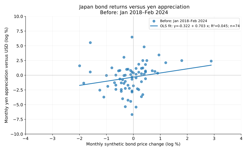
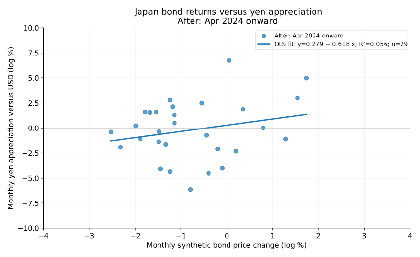
The fitted monthly relationship between bond-price changes and yen appreciation remains weak. Before the transition, its slope is approximately 0.703 with R² of 0.045 across 74 months. Afterward, the slope is approximately 0.618 with R² of 0.056 across 29 months. The positive slopes indicate a modest tendency for bond-price increases to coincide with yen appreciation in each sample. The small R² values show how much variation remains outside that simple relationship.
This does not demonstrate a clean transfer of volatility from bonds to currency. Both volatility measures increase, while the contemporaneous return relationship stays weak. Nor can the increases be attributed solely to the BOJ decision. US rates, inflation, positioning and other developments changed, the periods are unequal, and policy itself responds to economic conditions. A before-and-after comparison gives us a useful description of different environments, not an isolated estimate of the policy's causal effect.
For the blog's central argument, the result is valuable precisely because it requires care. It shows that public risk management cannot be assessed with one stable price, one debt ratio or one fitted line. It also shows why traders distinguish a hypothesis about the source of risk from an observed association between two returns. A thoughtful policymaker should make the same distinction before using a chart to justify a decision.
12. Rates, currencies and the location of adjustment
The old market expression that one can control rates or the currency, but not both, captures a real tension while omitting important conditions. The monetary trilemma concerns the compatibility of a fixed exchange rate, independent monetary policy and free capital mobility. Capital restrictions and intermediate exchange-rate arrangements complicate the comparison. IMF research discusses how policy rates and FX intervention interact with external tightening under different regimes.5
For our purposes, the useful question is where adjustment occurs when a policy limits movement in a particular price. A hypothetical government supporting an exchange rate might face different reserve, funding or domestic-credit consequences from one allowing that exchange rate to float. A central bank stabilizing long-term bond prices could alter the environment for investors' positioning. These possibilities are mechanisms to examine. They are not a rule requiring an equal and opposite movement in volatility elsewhere.
Political policymakers need this perspective because an intervention's visible success may not summarize its complete consequences. A stable price can be an intended and worthwhile outcome. Its evaluation should also consider the resources required to maintain it, how expectations change, and what happens under unfavorable conditions. The relevant comparison includes the costs of alternatives. Asking these questions does not imply that all intervention is harmful or that the least managed market is always the best policy outcome.
China offers a prospective extension centered on suppressed yuan volatility. The question is whether currency stability accompanies adjustment in bond prices, domestic credit, capital flows or official balance sheets. China is not in this thirteen-country sample, and our results establish none of those effects. A serious extension would need appropriate currency and bond data, policy dates and measures of the alternative adjustment channels before drawing conclusions about Chinese institutions or decisions.
13. What a more thoughtful policy discussion would require
A Merton-informed policy discussion begins by separating the size of obligations, the expected value of supporting resources, and uncertainty about those resources. It then asks how those elements respond together to a shock. A hypothetical recession may weaken revenues while raising demands for support. A financing disruption may affect commitments differently depending on their maturity and currency. The assessment should identify these dependencies rather than assuming that each exposure can be evaluated independently.
This approach would make fiscal communication more concrete. Political leaders could explain why a commitment is expected to strengthen future capacity, what would undermine that expectation, and what flexibility remains if outcomes disappoint. Central bankers could describe the objective of market stabilization alongside the conditions under which its operation would change. These are demanding questions, but they are more informative than alternating between blanket reassurance about debt and blanket declarations that a particular ratio is intolerable.
The distribution of losses also deserves explicit attention. The simplified model allocates losses between corporate claims. Public policy must consider households, taxpayers, pensioners, workers and firms, whose exposures differ. Meeting a nominal payment does not settle the entire economic question. Nor does avoiding a nominal default prove that the adjustment was equitable or inexpensive. A financially thoughtful policy discussion should identify who is exposed in each scenario and which public objectives justify accepting those exposures.
There is a constructive role for borrowing and stabilization within this framework. Preserving employment, maintaining essential services or investing in productive capacity can improve the distribution of future outcomes. Risk awareness should help policymakers distinguish sound commitments from fragile ones, not become an excuse for neglecting public needs. The derivatives analogy is most useful when it encourages preparation for uncertainty and clearer accounting of consequences, while leaving democratic judgment about objectives where it belongs.
14. What we can conclude—and what we should test next
Our strongest descriptive cross-section is the relationship between debt/GDP and German-relative spreads within six euro-area borrowers. Across the broader country set, debt/GDP explains little bond volatility. Currency results vary sharply between a five-country snapshot and historical pooled observations. Japan shows higher bond and yen volatility after the selected policy transition, but weak monthly return relationships on both sides. Each finding contributes to the argument without providing a single comprehensive explanation of sovereign risk.
The next empirical work should use fiscal-resource proxies, maturity and currency composition, and measures of contingent liabilities. Country effects and common global factors would improve the historical comparisons. Comparable daily bond data would permit daily bond-volatility estimates without interpolation. Equal-length policy windows, rolling measures and sensitivity to alternative boundaries would help assess the Japan comparison. Inference would also need to account for repeated observations, serial dependence and the small number of countries.
The Merton chart remains important because it changes the questions we ask. Its curves illustrate how leverage and uncertainty can interact nonlinearly under stated assumptions. They do not establish that risk begins at 100 percent debt/GDP, nor do they tell us which country will experience a crisis. Their policy value lies in making hidden sensitivities visible and showing why a calm present can coexist with a more vulnerable range of future outcomes.
That is the case for central bankers thinking like derivatives traders, and for political policymakers learning the same discipline. Examine the exposure before celebrating its price. Examine the unfavorable states before relying on the central forecast. Examine the full set of public consequences before concluding that an obligation has been safely managed. The aim is a policy conversation capable of understanding uncertainty, preparing for it, and explaining its choices honestly to the people who ultimately bear the risk.
References and replication notes
- Merton, Robert C. (1974). “On the Pricing of Corporate Debt: The Risk Structure of Interest Rates.” The Journal of Finance 29(2), 449–470. Published paper and DOI. MIT working-paper predecessor.
- Gray, Dale F., Robert C. Merton and Zvi Bodie (2007). “Contingent Claims Approach to Measuring and Managing Sovereign Credit Risk.” Journal of Investment Management 5(4). Journal issue and abstract.
- Gapen, Michael T., Dale F. Gray, Cheng Hoon Lim and Yingbin Xiao (2008). “Measuring and Analyzing Sovereign Risk with Contingent Claims.” IMF Staff Papers 55, 109–148. DOI. IMF abstract.
- Bank of Japan (19 March 2024). Changes in the Monetary Policy Framework. For institutional responsibility for FX intervention, see the BOJ's explanation of Ministry of Finance instructions and BOJ execution.
- Huertas, Gonzalo (2022). Why Follow the Fed? Monetary Policy in Times of U.S. Tightening. IMF Working Paper 2022/243. Used for the conditional trilemma and interaction of monetary/FX tools, not as evidence for our regression results.
- International Monetary Fund, World Economic Outlook / Data Mapper. General-government gross debt, percent of GDP (GGXWDG_NGDP). Snapshot retrieved 3 October 2026; historical values may include estimates and revisions. Current and future calendar years were excluded from the supplied snapshot. This cutoff does not establish that all retained values are final actuals.
- FRED/OECD monthly ten-year yield series: IRLTLT01{country}M156N for US, IT, FR, GR, ES, DE, JP, CA, CH, IE, NL, DK and AU. Example: Japan ten-year yields. FX series: DEXUSEU, DEXJPUS, DEXCAUS, DEXSZUS, DEXDNUS and DEXUSAL. Example: JPY per USD. Quotations are normalized to USD per local currency for the analysis.
All regressions are descriptive OLS with an intercept. Debt/GDP scatters merge linear and degree-2 fits on the same observations; return-versus-return regressions retain their linear fits. Adjusted R² comparisons are reported in the text where discussed. No significance tests or causal estimates are claimed. The archive includes chart data from the inspected operator output, SVGs, the command, the debt snapshot, and a Python chart-generation script. The scenario table is independently recomputed from the stated equations. Graphs are publication redraws of the operator data; the Japan scatter axes are identical. The full sample remains visible. Figure 3b is an explicitly labeled sensitivity comparison excluding Japan; both snapshot charts use identical axes.