The Tolstoy Problem
What the unemployment rate doesn't tell us—and why the labor market can appear stable while millions of people move beneath the surface.
Economists frequently turn to the Beveridge curve when discussing the labor market. It relates the unemployment rate to the job-vacancy rate. When employers have openings to fill, unemployment generally falls. When vacancies disappear, unemployment usually rises.
On a chart, the relationship looks reassuringly simple. It slopes downward. We use it to discuss labor-market tightness, matching efficiency, monetary policy, and the possibility of a soft landing.
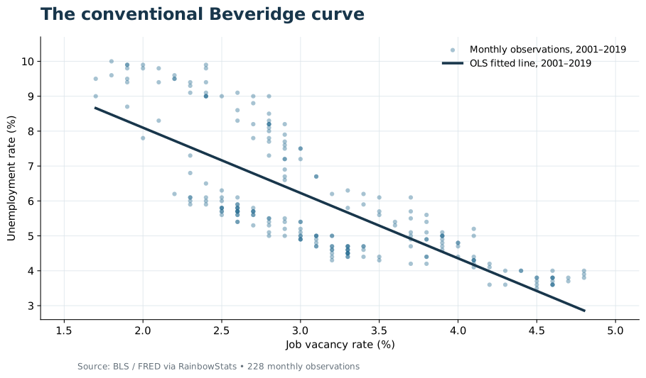
But there is a problem. The curve moves.
A relationship, not a law
During the Great Recession the economy followed one path. During COVID it went somewhere else entirely. After 2022, the unemployment–vacancy relationship looked different again. We can draw a fitted curve through each period, but that doesn't make the relationship permanent.
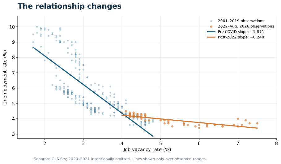
Using RainbowStats, I estimated two simple regressions with unemployment as the dependent variable and vacancies as the explanatory variable:
| Period | Vacancy coefficient | R² | Observations |
|---|---|---|---|
| 2001–2019 | −1.871 | 0.598 | 228 |
| 2022–Aug. 2026 | −0.240 | 0.631 | 55 |
That's quite a change in the descriptive slope. Yet the estimated relationships show persistent residuals: the Durbin–Watson statistics are only 0.076 and 0.355, respectively. We should not confuse a good fit, or a difference in fitted slopes, with a complete explanation of the labor market.
Lost in the forest
I tried increasingly complex statistical approaches: rolling regressions, structural breaks, participation-rate interactions, transfer functions, and corrections for autocorrelation. There is useful information in those methods. Yet I began to feel we were getting lost in the forest of regressions.
Consider a worker retiring from a full-time career and returning to a part-time job in retail. Is that a retirement? A job change? A response to inadequate savings? Perhaps all three. Through much of the transition, that person may never count as unemployed.
Average weekly hours added information to our vacancy model; an interaction between hours and vacancies was statistically strong in the full sample. But even that regression could not identify the worker's reason for accepting fewer hours. Nor did the model resolve persistent residual autocorrelation.
What we see in the aggregate is not the full story.
Enter Tolstoy
In War and Peace, Leo Tolstoy questions whether we can explain history through the decisions of a handful of famous individuals. History, in his telling, grows out of countless human choices, each made in its own circumstances.
The labor market works much the same way. Millions of people take jobs, leave jobs, retire, return to employment, attend school, care for family members, or find themselves looking for work. The unemployment rate compresses those decisions into a single statistic.
To see what we were missing, I returned to an earlier RainbowStats labor-flow model. Instead of counting people in each category, it tracks their monthly transitions among three states: employed, unemployed, and outside the labor force.
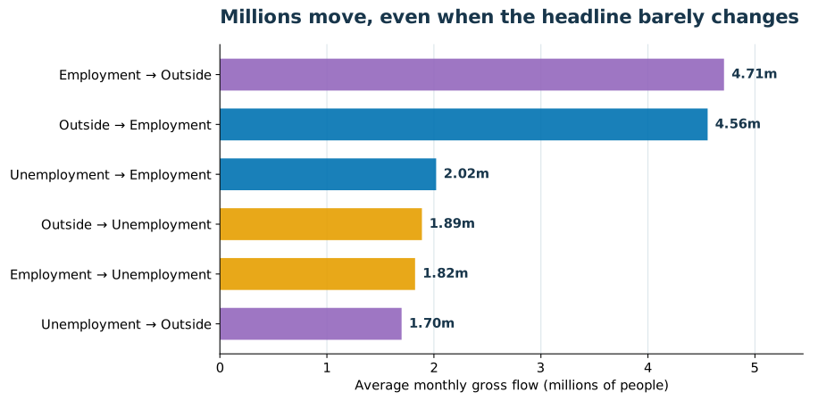
On average, around 4.7 million people moved from employment to outside the labor force each month, while around 4.6 million moved in the opposite direction. The flows were enormous, and they frequently offset one another.
Even those six paths leave part of the story untold. They do not distinguish a retired engineer taking a part-time retail job from a parent returning to work, nor do they distinguish full-time from part-time employment.
Watch the labor market move
The animated Sankey below displays monthly labor-market transitions from January 2018 through September 2026. Each colored ribbon represents a particular movement; its width reflects the number of people making that transition. Colors remain consistent from month to month.
This is the visualization that changed how I thought about the problem. The familiar unemployment rate may barely budge while millions of people are moving in and out of employment.
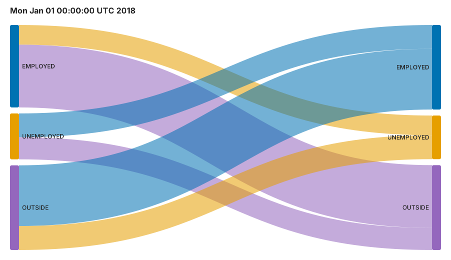
If the animation does not play in your reader or an email preview, open the SVG directly in a modern browser.
What looks like equilibrium from a distance may be the outcome of extraordinary movement underneath.
The Beveridge curve remains useful. Regressions remain useful. But Tolstoy offers a warning: a compressed description of millions of individual actions is not the same as understanding them. Sometimes the best next step is not another regression. It is to watch the people move.