Who Controls Interest Rates?
The Federal Reserve, economic growth, and the feedback loop between Treasury yields, investment, and consumption.
The Federal Reserve can influence interest rates. But can it control them?
That question sounds almost heretical in a world where every Federal Reserve announcement is examined for clues about borrowing costs. Markets move on the slightest change in language from the Federal Open Market Committee. Yet the Federal Reserve directly controls neither the ten-year Treasury yield nor all the economic forces that determine it.
The ten-year yield reflects expectations about growth, inflation, future short-term rates, Treasury borrowing, and the compensation investors require for holding long-term bonds. Monetary policy matters. So do the economy and the market.
Our original question was straightforward: Do higher interest rates necessarily reduce economic activity? Our revised analysis asks another question: What happens to interest rates when economic growth accelerates?
The conventional view of interest rates
The familiar story begins with higher interest rates, more expensive borrowing, delayed investment, and slower spending. Lower rates are expected to reverse the sequence.
But higher interest rates also increase income for some holders of interest-bearing assets. Government interest payments are an expense to the Treasury and income to bondholders. The ultimate economic effect depends on who receives that income, who bears the financing costs, and how they respond.
Timing matters. Newly issued Treasury debt reprices immediately; the government's overall interest expense adjusts more gradually as outstanding debt matures. The economy is a system of interacting relationships, not a single equation.
A challenge to the conventional mechanism
Our investigation was partly motivated by Justin Bloesch and Jacob P. Weber's March 2026 Federal Reserve Bank of New York study, Structural Changes in Investment and the Waning Power of Monetary Policy. Their work investigates how changes in the structure of investment may weaken the transmission of monetary policy to labor income and consumption. Read the staff report.
If the structure of the economy changes, perhaps we should reconsider not only the strength of monetary-policy transmission but also the directions in which interest rates and economic activity influence each other.
A system of economic relationships
We assembled quarterly observations beginning in 1980, using real investment growth, real consumption growth, real GDP growth, changes in the ten-year Treasury yield, and changes in federal interest payments relative to GDP. A separate investment model adds federal debt and corporate indebtedness.
We estimated four simultaneous relationships: investment depends on growth, yields, and interest payments; consumption depends on growth and financing conditions; GDP depends on investment and consumption; and the federal interest burden depends on yields and GDP.
These equations describe a feedback system. Investment contributes to GDP, while GDP supports investment. Consumption contributes to production, while income supports consumption. Interest rates affect financing costs, while economic growth affects interest-rate expectations.
Seeing the system: the Sankey diagram
The Sankey diagram is the central visual in this investigation. It makes the interdependence of the simultaneous equations visible at a glance.
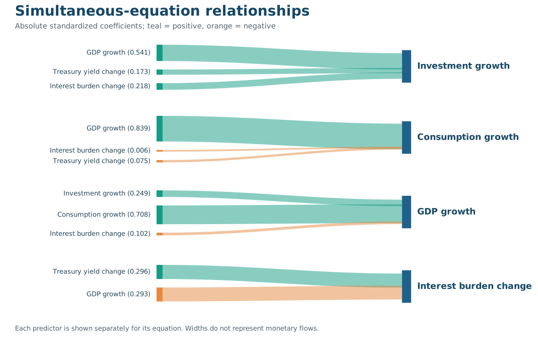
A regression table contains coefficients and standard errors. The Sankey diagram communicates something else: the interconnected nature of the economic system. Monetary policy does not operate on an isolated investment decision. It operates within a network of spending, production, financing costs, and interest income.
Federal debt and the investment response
Federal debt introduces another dimension. When outstanding debt is large, changes in market yields may eventually produce larger changes in government interest expense. That does not establish that higher rates stimulate the economy, but it raises a testable question about income distribution and the stock of debt.
We estimated a quadratic distributed-lag model of investment growth, allowing the effect of nine quarterly Treasury-yield changes to vary with lagged federal debt relative to GDP. We examined ordinary least squares, HAC standard errors, residual autocorrelation, and Wald restrictions.
The earlier joint debt-interaction test had a p-value of approximately 0.139; the cumulative restriction had a p-value of approximately 0.074. These are suggestive rather than decisive results. Indebtedness may alter the investment response, but our evidence does not establish that conclusion at the conventional 5% significance level.
The missing direction of causality
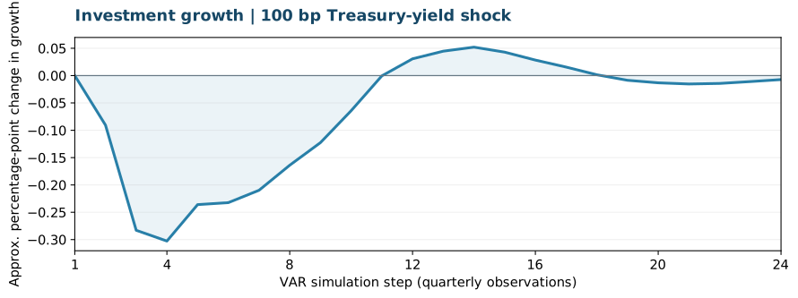
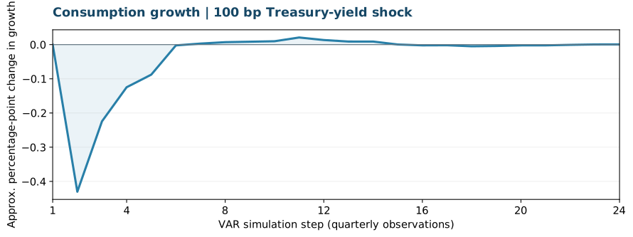
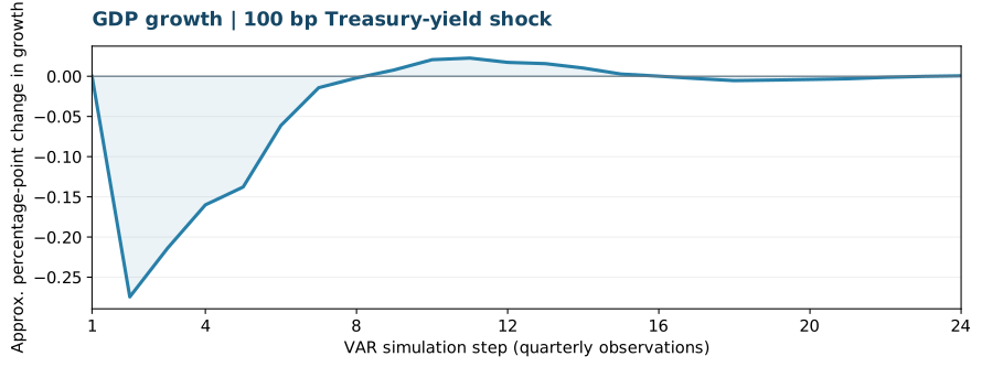
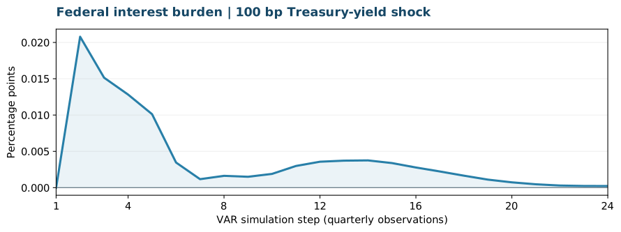
We then estimated a five-variable vector autoregression with four quarterly lags. The first experiment shocked the ten-year Treasury yield. Investment, consumption, and GDP growth initially weakened, while the federal interest burden increased.
Then we reversed the question. Instead of asking what yields do to growth, we asked what stronger GDP growth does to yields.
Interest rates are not simply an instrument acting upon the economy. They are also an outcome of economic activity.
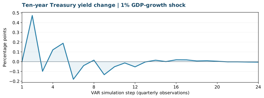
A positive innovation of 0.01 log points in real GDP growth produced a subsequent positive response in the ten-year Treasury yield change, reaching approximately 47 basis points in the early response sequence. The response then oscillated.
This is a model simulation, not evidence that every one-percentage-point increase in GDP growth necessarily raises yields by 47 basis points. It depends on the fitted VAR and the definition of the shock. Nevertheless, it illustrates the two-way nature of the relationship.
What this means for monetary policy
A rise in long-term yields may reflect expectations of tighter monetary policy. But it might also reflect stronger anticipated growth, higher expected inflation, increased Treasury issuance, or a higher term premium. These explanations are economically different.
Our VAR does not fully identify those components. It estimates historical dynamic relationships. Still, the two experiments reinforce an important distinction: higher yields can weaken growth, and stronger growth can raise yields.
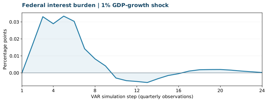
The Sankey diagram illustrates contemporaneous feedback in the estimated system. The VAR illustrates how disturbances propagate through that system over time. The full numerical shock analysis appears in the appendix.
Conclusion: the Fed does not operate in a vacuum
The Federal Reserve controls its short-term policy-rate target and can influence longer-term yields through expectations and balance-sheet policy. But the ten-year Treasury yield is a market price, shaped by investors' assessments of economic conditions.
Our analysis finds responses in both directions: higher yields initially weaken real growth in the fitted model, while stronger GDP growth initially raises Treasury yields. Federal debt and interest-income feedback remain promising questions for further study, not settled conclusions.
Perhaps the most important lesson is methodological. An economy cannot be understood through one regression coefficient, one interest rate, or one policy announcement. It is a system of feedback relationships. Sometimes the most revealing experiment is to reverse the direction of the question.
Appendix · Data, models, and complete shock analysis
A. Data and transformations
| FRED series | Variable | Transformation |
|---|---|---|
| PNFI | Private nonresidential fixed investment | Deflate by GDPDEF; log difference |
| GDPDEF | GDP implicit price deflator | Deflator |
| GDP | Gross domestic product | Deflate by GDPDEF; log difference |
| PCE | Personal consumption expenditures | Deflate by GDPDEF; log difference |
| GS10 | Ten-year Treasury yield | Quarterly conversion; first difference |
| GFDEGDQ188S | Federal debt/GDP | Lagged ratio |
| A091RC1Q027SBEA | Federal interest payments | Divide by GDP; first difference |
| BOGZ1FA106130003Q | Corporate debt measure | Relative to GDP |
B. Simultaneous equations
Consumption growth = f(GDP growth, interest burden change, yield change)
GDP growth = f(investment growth, consumption growth, interest burden change)
Interest burden change = f(yield change, GDP growth)
The system uses lagged variables as candidate instruments. The three-stage implementation is an IV/SUR approximation; instrument relevance, exclusion restrictions, and identification require further validation.
three = THREE_STAGE_REGRESSION(system,instruments)
sankey = EXTRACT(three,"sankey")
var4 = EXTRACT(three,"varmodel:4")
C. Five-variable VAR(4)
The variable order is: (0) Treasury yield change; (1) real investment growth; (2) real consumption growth; (3) real GDP growth; (4) interest burden change.
v = VAR_MODEL(LIST(dr,g,gc,gy,dj),4)
Shock responses are the difference between a recursively simulated shocked forecast and its unshocked baseline. The experiment uses additive shocks in the units of the estimated series, not identified structural monetary-policy innovations. No uncertainty bands are estimated.
D. Experiment 1: +100-basis-point Treasury-yield shock
rate_to_investment = EXTRACT(v,"shockdiff:1:0:1")
rate_to_consumption = EXTRACT(v,"shockdiff:2:0:1")
rate_to_gdp = EXTRACT(v,"shockdiff:3:0:1")
rate_to_interest = EXTRACT(v,"shockdiff:4:0:1")
| Response | Minimum | Maximum |
|---|---|---|
| Investment growth (log points) | −0.003027 | +0.000521 |
| Consumption growth (log points) | −0.004302 | +0.000208 |
| GDP growth (log points) | −0.002744 | +0.000226 |
| Interest burden change (percentage points) | 0.000000 | +0.020787 |
The negative growth-rate extrema correspond to approximately 0.30%, 0.43%, and 0.27% lower investment, consumption, and GDP growth rates relative to baseline. They are not equivalent declines in the levels of those variables.
E. Experiment 2: positive real GDP-growth shock
growth_to_rate = EXTRACT(v,"shockdiff:0:3:0.01")
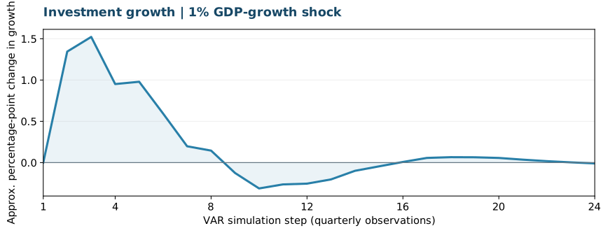
growth_to_investment = EXTRACT(v,"shockdiff:1:3:0.01")
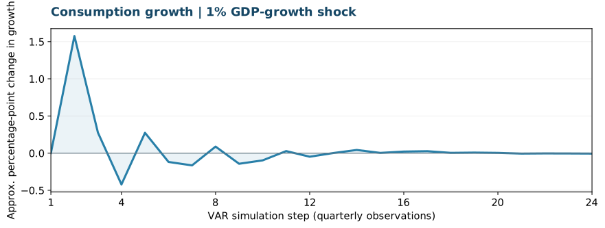
growth_to_consumption = EXTRACT(v,"shockdiff:2:3:0.01")
growth_to_interest = EXTRACT(v,"shockdiff:4:3:0.01")
A +0.01-log-point innovation is approximately a one-percentage-point increase in quarterly log growth.
| Simulation step | Yield-change response (percentage points) |
|---|---|
| 1 | 0.0000 |
| 2 | +0.4729 |
| 3 | −0.0987 |
| 4 | +0.1213 |
| 5 | +0.1885 |
| 6 | −0.1805 |
| 7 | −0.0402 |
| 8 | +0.0156 |
| 9 | −0.1335 |
The zero response in step 1 is consistent with a lagged VAR: the GDP-growth innovation enters the yield equation through lagged values, so the first yield response appears in step 2. The full simulation returns 24 observations.
F. Debt-dependent distributed-lag tests
The investment regression summarizes nine quarterly Treasury-yield changes with a quadratic polynomial and interacts those terms with lagged federal debt/GDP. Controls include GDP growth, lagged investment growth, and corporate indebtedness.
| Restriction | Chi-square | df | p-value |
|---|---|---|---|
| Joint debt interactions | 5.4896 | 3 | 0.1393 |
| Cumulative debt interaction | 3.1964 | 1 | 0.0738 |
These earlier results are exploratory. They do not establish a debt-dependent effect at the conventional 5% significance threshold. Supporting OLS, HAC, residual autocorrelation, and actual-versus-fitted charts are available in the linked slideshow.
G. Limitations and next steps
- VAR innovations are not necessarily structural monetary-policy shocks.
- Shock magnitudes are additive in series units, not standardized by innovation variance.
- The current implementation does not provide impulse-response confidence bands or a formal stability assessment.
- Federal interest payments are not identical to interest income received by domestic households.
- GDP includes investment and consumption, creating accounting relationships among modeled variables.
- The simulation date routine currently advances displayed dates by approximately 30 days per step, even though the underlying VAR observations are quarterly. Interpret the horizontal axis as model periods until that routine is corrected.
Potential extensions include the federal funds rate, inflation expectations, Treasury term-premium estimates, credit conditions, structural VAR identification, and local projections.