From Magic to Alchemy | RainbowStats

“Being stupid with dummy variables” is memorable, but it blames the tool. Dummy variables are not stupid. The mistake is asking a long list of historical regimes to explain the past and then treating the resulting fit as if it identified an economic mechanism.

This experiment deliberately walks toward that trap. We estimate two relationships in levels, add tax-policy period dummies, repeat everything in log differences, and finally inspect the residual correlograms. The point is not that policy dummies should never be used. The point is that a model can become more impressive and less informative at the same time.

The test: If tax-policy regimes genuinely clarify the relationship, they should improve more than raw in-sample fit. The key coefficient should remain stable, adjusted fit and information criteria should improve, and residual structure should become more credible without consuming the model’s degrees of freedom.

Act I: Inequality and corporate profits

The first regression compares the U.S. Gini index with corporate profits as a share of GNP. In levels, both series carry decades of history. That makes the chart interesting—but also makes ordinary least squares vulnerable to shared trends, structural breaks, and omitted variables.

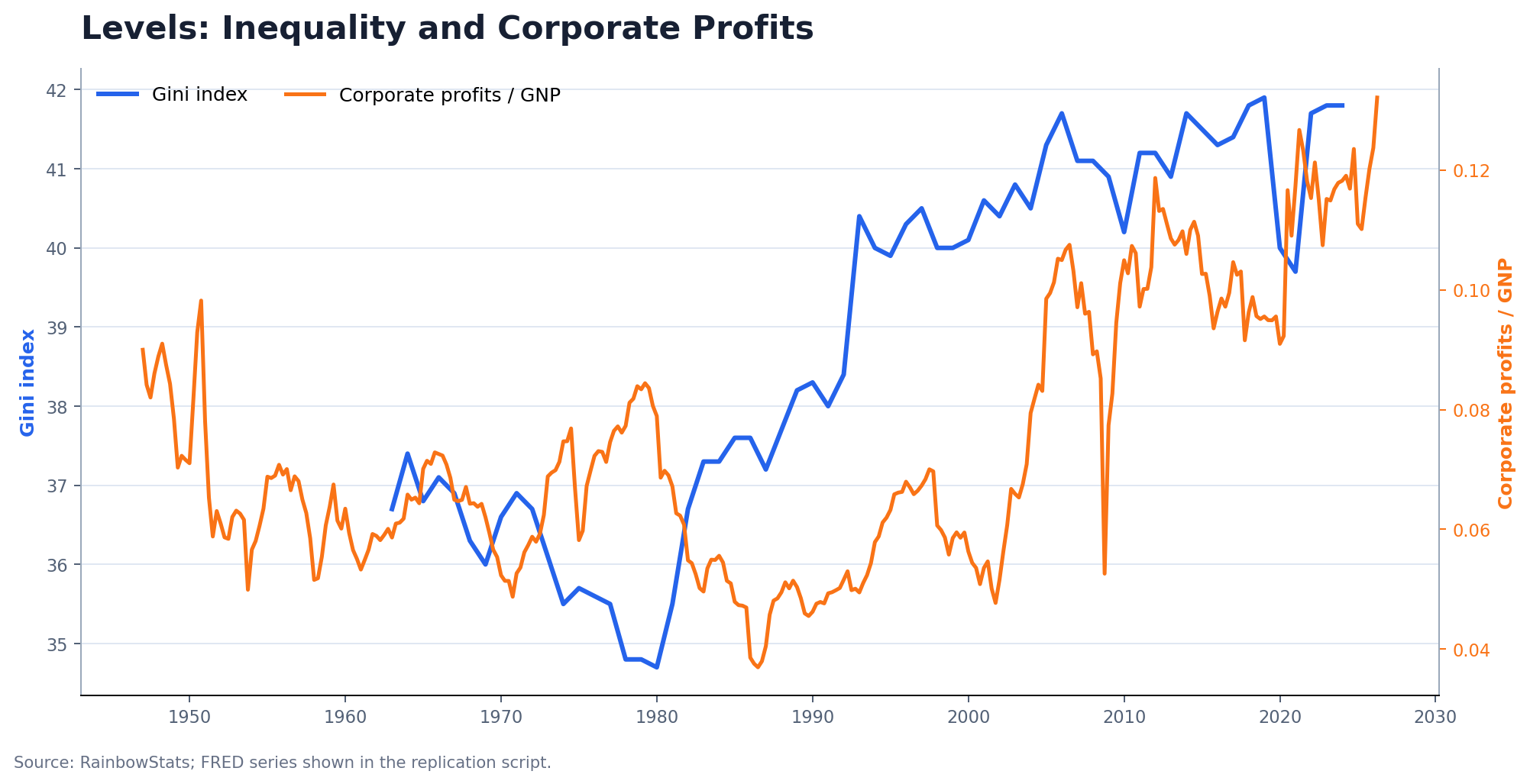
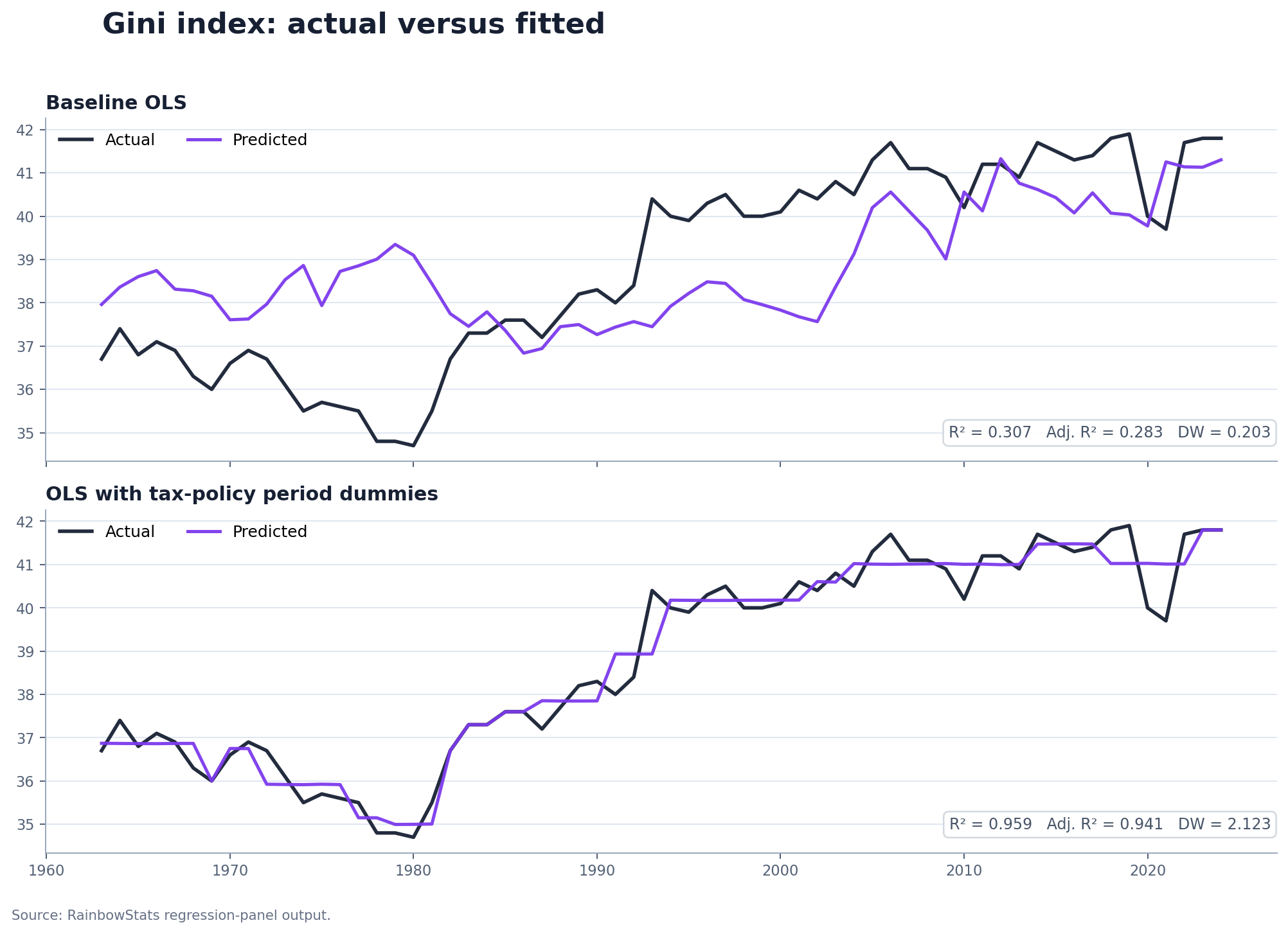
Dual-axis chart of the U.S. Gini index and corporate profits as a share of GNP — **Figure 1.** The levels move together over parts of the sample, but co-movement across long historical spans is not itself a causal mechanism.

The baseline levels regression produces R²=0.307. The profit-share coefficient is 56.057 with a t-statistic of 5.151. Add 16 tax-policy period dummies and the fit jumps to R²=0.959. Yet the coefficient on corporate profits collapses to −0.630 with a t-statistic of −0.063.

0.307 → 0.959Levels R² after adding tax regimes

5.151 → −0.063Profit-share t-statistic

56.057 → −0.630Profit-share coefficient

That is the central warning. The model fits inequality extremely well only after the calendar regimes take over the explanatory work. What has been “explained” is not necessarily a tax-policy channel. The regimes can also proxy for inflation, recessions, technology, labor-market institutions, demographics, globalization, or any other force that moved over the same periods.

Actual and fitted Gini index under baseline OLS and dummy-variable OLS — **Figure 2.** The dummy model hugs the historical Gini path. Its visual precision coincides with the disappearance of the corporate-profit coefficient.

The autocorrelation evidence

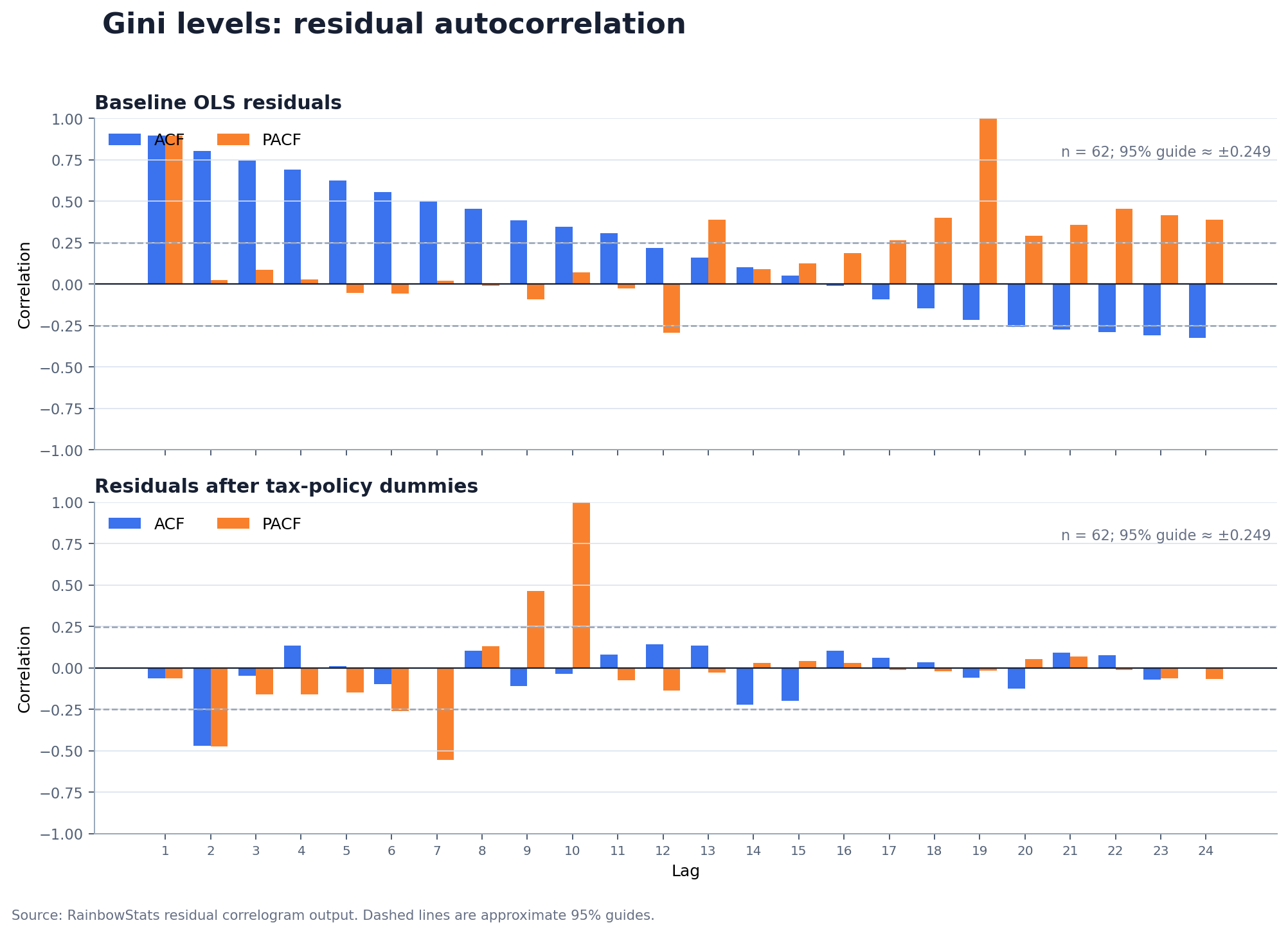
The baseline levels residuals are profoundly persistent: the lag-one residual ACF is 0.895 and the Durbin–Watson statistic is 0.203. The dummy model largely absorbs that long structure and raises Durbin–Watson to 2.123. This is a better residual picture—but it was achieved by giving 62 annual observations 16 policy-regime indicators. The fit describes the sample very closely; it does not identify why the regimes line up with inequality.

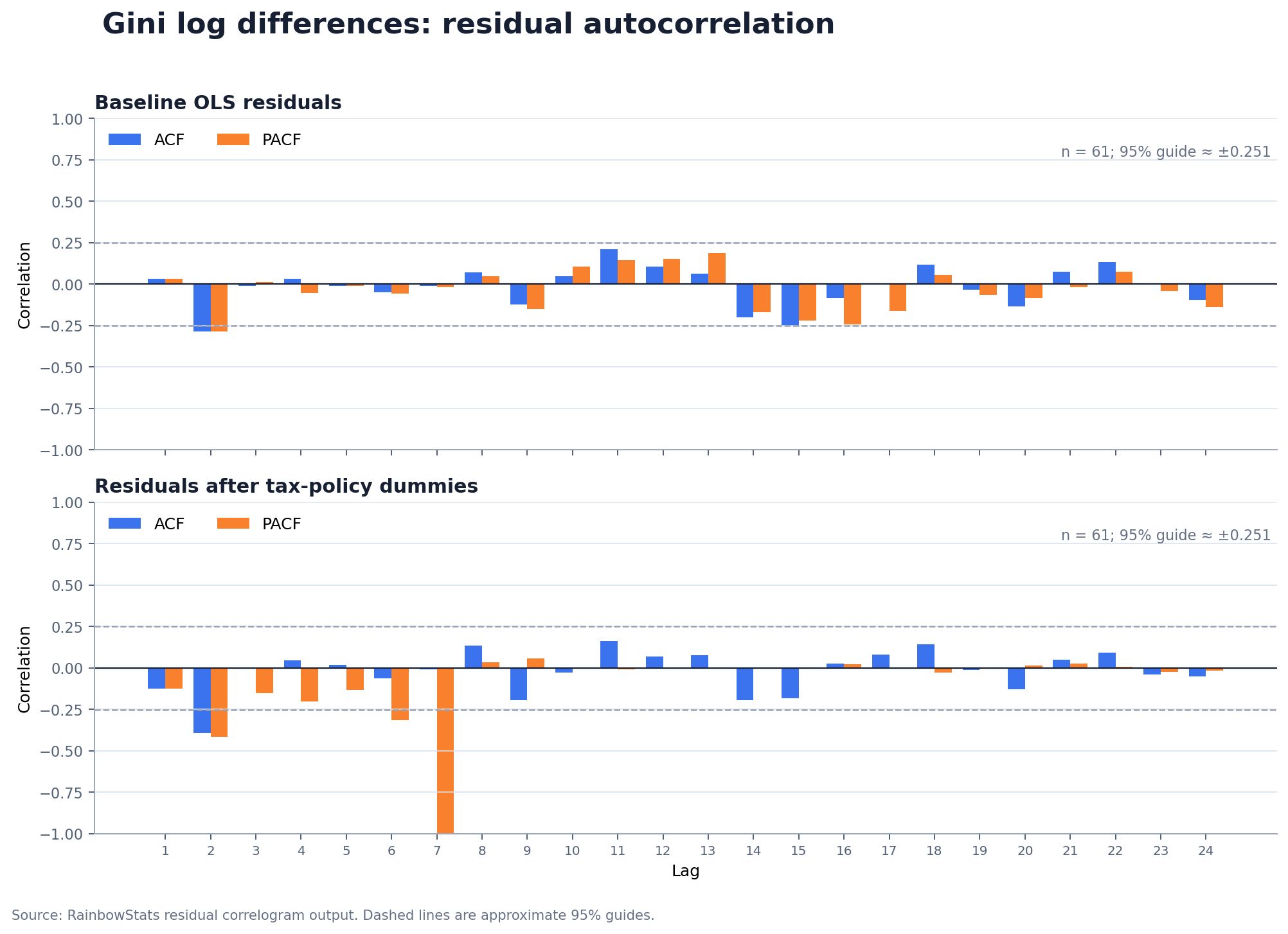
ACF and PACF of Gini levels regression residuals before and after tax-policy dummies — **Figure 3.** Tax-period dummies remove much of the slow residual persistence in the levels model. That demonstrates their power to segment history, not proof that tax legislation caused the segmented path.

Log differences provide the harder test. Once persistence is removed, the baseline relationship shrinks to R²=0.038, adjusted R²=0.0045, and a profit-growth t-statistic of −1.519. Adding the dummies raises raw R² to 0.220, but adjusted R² falls to −0.114 and the model F-statistic falls to 0.715. AIC worsens from −505.844 to −486.681, while BIC worsens from −501.623 to −448.685.

ACF and PACF of Gini log-difference regression residuals before and after tax-policy dummies — **Figure 4.** Differencing removes most of the persistence before the policy dummies are added. The extra regimes buy raw fit but fail the penalty for complexity.

Act II: Tax receipts and nominal GDP

The second example is almost built to look good. Federal current tax receipts and nominal GDP both rise with the size of the economy and the price level. A levels regression therefore delivers R²=0.984 before any policy dummies are introduced.

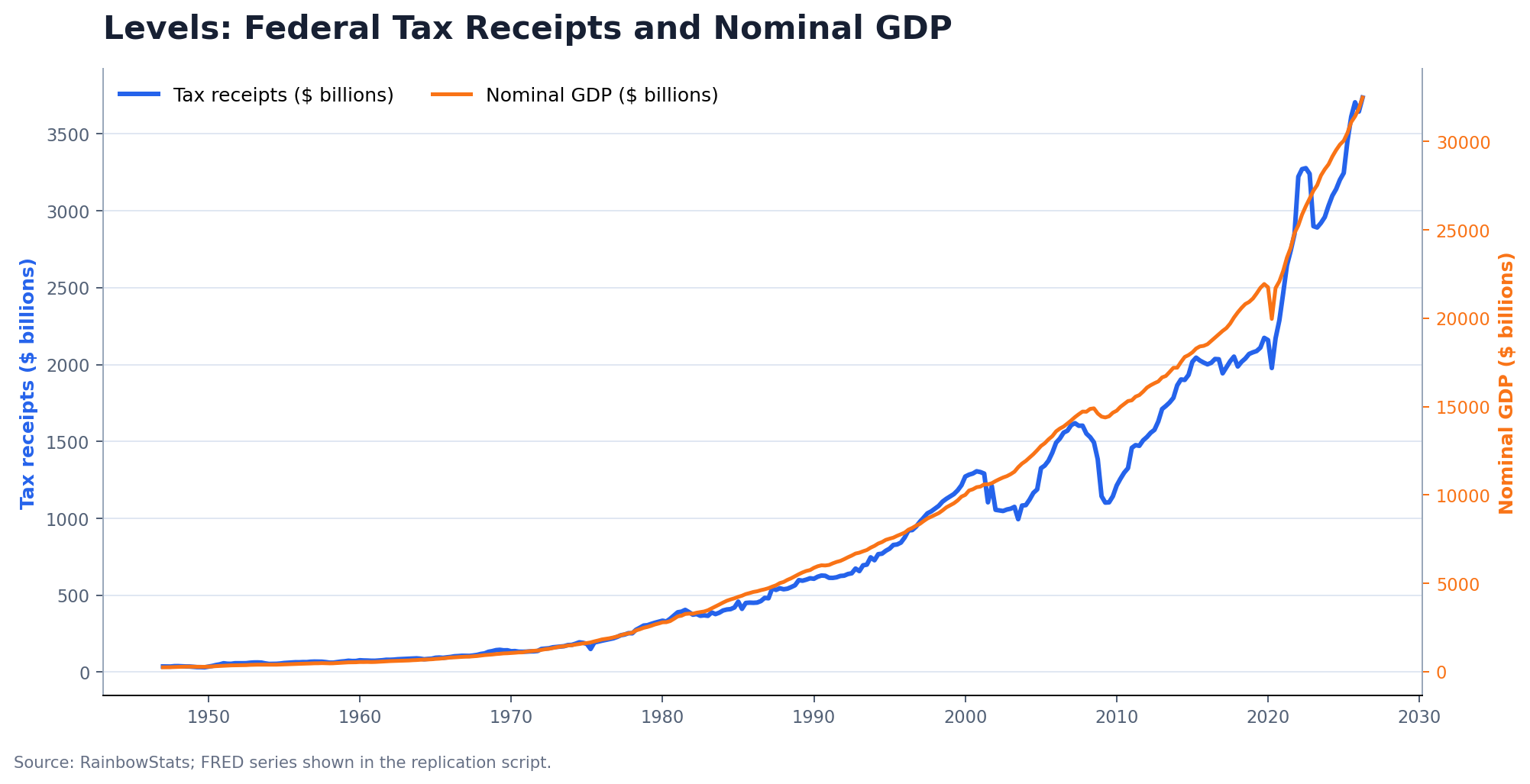
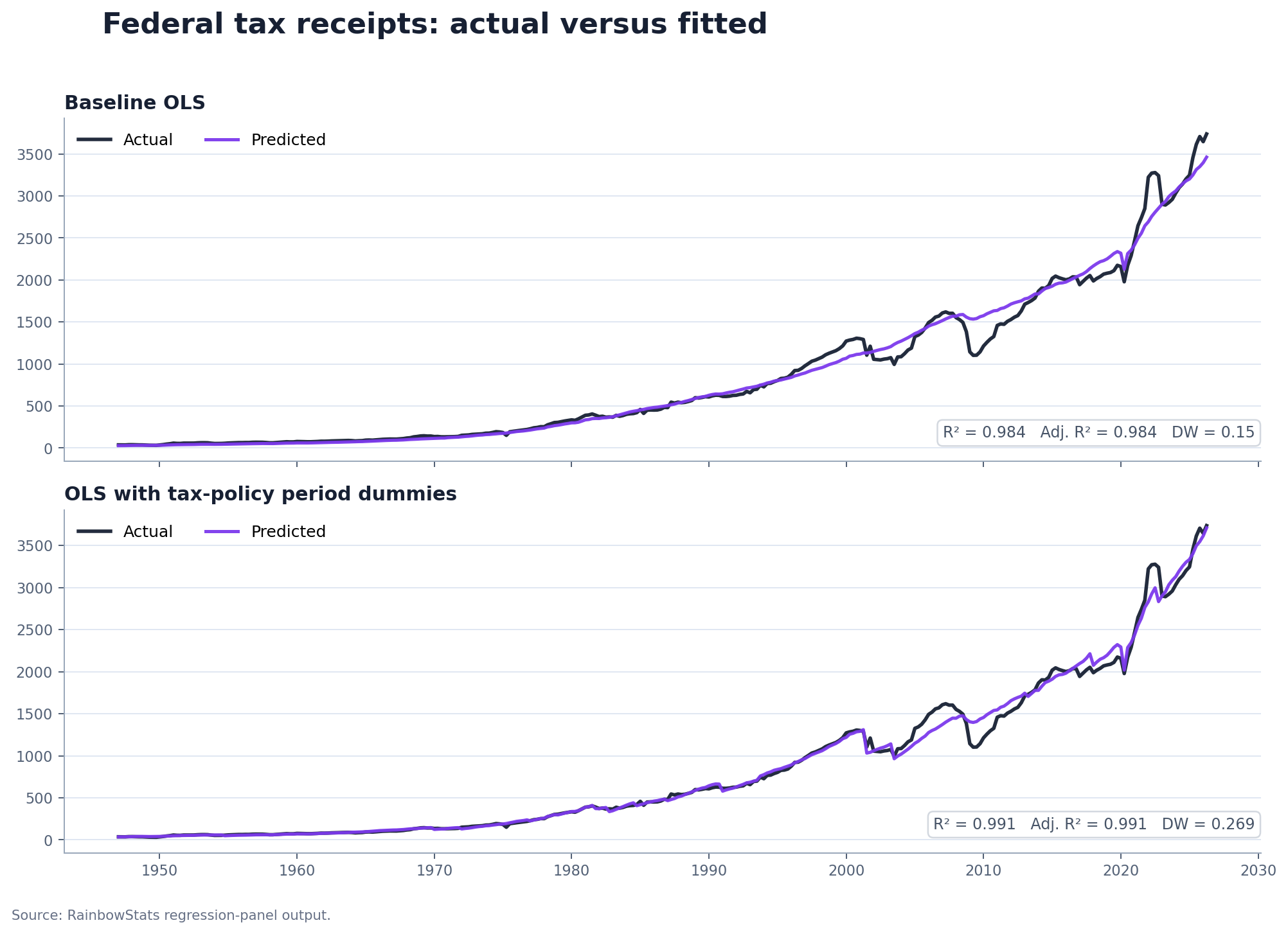
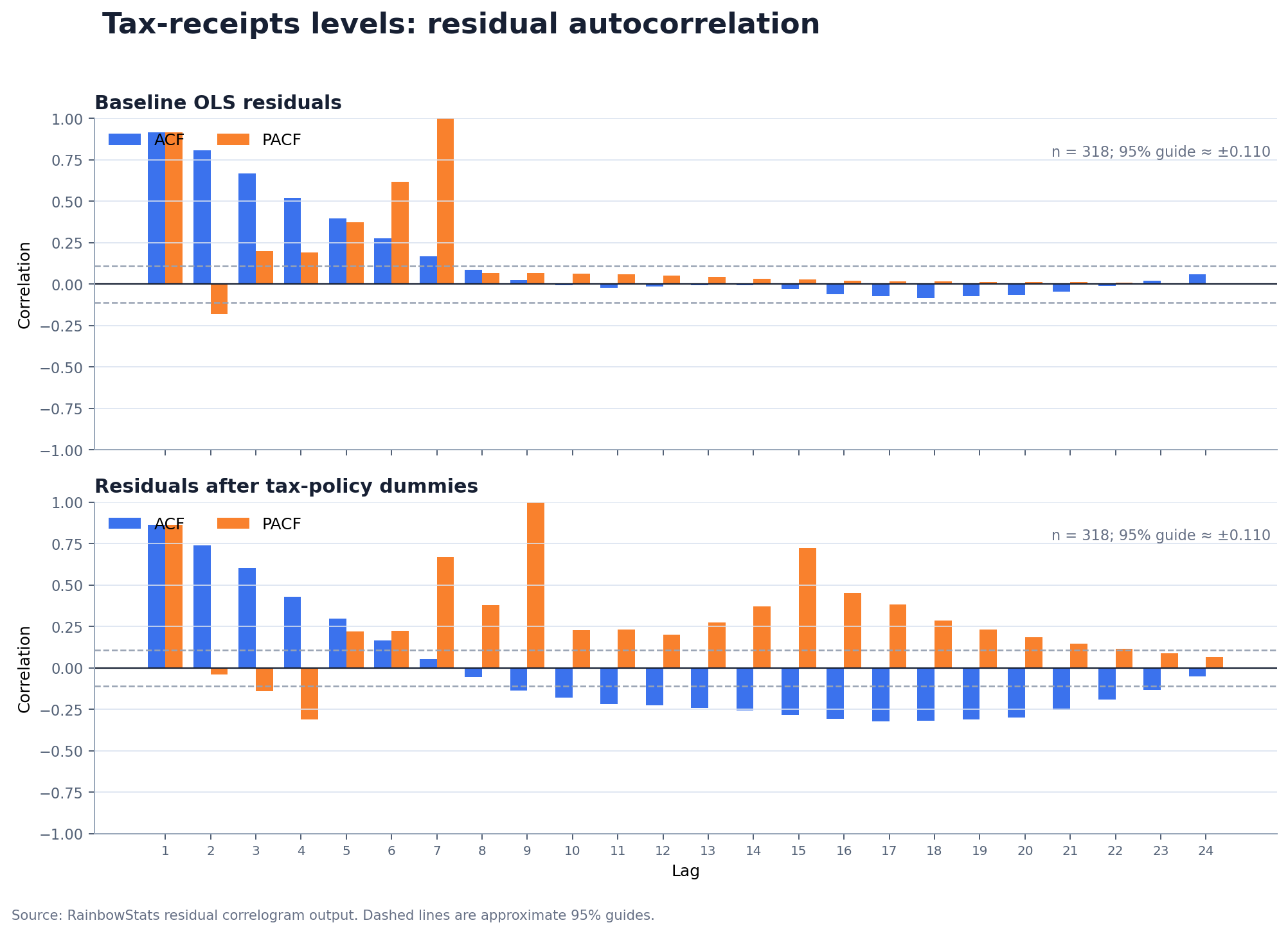
Dual-axis chart of federal current tax receipts and nominal GDP — **Figure 5.** Two nominal aggregates share an enormous long-run trend. A high levels R² is expected and should not be mistaken for a fully specified dynamic relationship.

Adding 17 tax-policy regimes raises (R²) from 0.984 to 0.991. That looks like an improvement, but residual persistence remains extreme: Durbin–Watson moves only from 0.150 to 0.269, and the lag-one ACF remains 0.865 after the dummies.

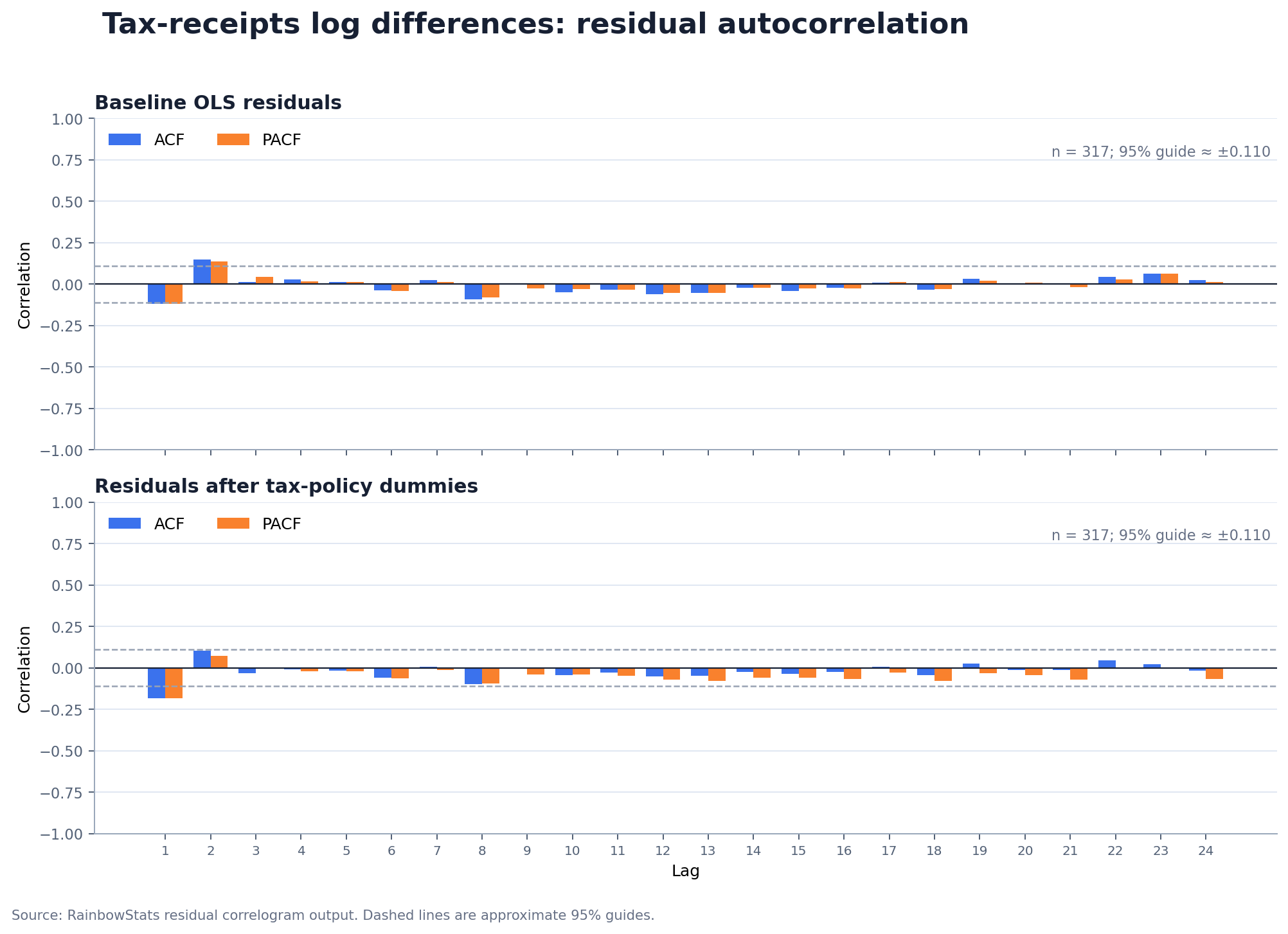
Actual and fitted federal tax receipts under baseline and dummy-variable OLS — **Figure 6.** Both levels specifications appear extraordinarily precise because GDP and receipts share the same nominal scale trend.

ACF and PACF of tax-receipts levels regression residuals before and after tax-policy dummies — **Figure 7.** The correlogram rejects the comforting visual story: the levels residuals remain strongly serially correlated even after adding tax regimes.

In log differences, GDP growth remains economically and statistically informative. The baseline coefficient is 1.780 with a t-statistic of 10.885; R²=0.273 and adjusted R²=0.269. Adding the policy dummies raises raw R² to 0.312, but adjusted R² slips to 0.268. AIC and BIC both worsen. The additional historical segmentation contributes almost nothing after complexity is properly penalized.

ACF and PACF of tax-receipts log-difference regression residuals before and after tax-policy dummies — **Figure 8.** Growth-rate residuals are already far closer to white noise. The dummy variables do not materially improve the dynamic specification.

All eight specifications

The complete comparison makes the pattern difficult to miss. Dummies reliably increase raw (R²), because that is what added regressors do. The meaningful question is what survives after accounting for lost degrees of freedom, parameter stability, and residual dynamics.

Relationship	Specification	R²	Adj. R²	DW	Key β	t-stat	AIC	BIC
Gini levels	Baseline	0.307	0.283	0.203	56.057	5.151	83.146	87.4
Gini levels	+ tax dummies	0.959	0.941	2.123	-0.63	-0.063	-59.598	-21.31
Gini log diff.	Baseline	0.038	0.0045	1.912	-0.025	-1.519	-505.844	-501.623
Gini log diff.	+ tax dummies	0.22	-0.114	2.208	-0.014	-0.712	-486.681	-448.685
Tax receipts levels	Baseline	0.984	0.984	0.15	0.106	139.239	3,013.82	3,021.34
Tax receipts levels	+ tax dummies	0.991	0.991	0.269	0.153	27.616	2,855.3	2,926.78
Tax receipts log diff.	Baseline	0.273	0.269	2.236	1.78	10.885	-2,090.33	-2,082.81
Tax receipts log diff.	+ tax dummies	0.312	0.268	2.363	1.871	10.518	-2,073.86	-2,002.44

What the experiment establishes

Levels can manufacture confidence. Trending or persistent variables often generate attractive fits and highly autocorrelated residuals.
Historical dummies can absorb almost any chronology. They may improve fitted values while replacing the economic relationship one intended to estimate.
Raw R² is not a model-selection rule. Adjusted R², AIC, BIC, residual autocorrelation, coefficient stability, and out-of-sample performance all matter.
A dummy variable is not a causal design. A policy date can coincide with many other structural changes.
Transformations change the question. Log differences ask whether changes move together, which is usually more demanding than asking whether two historical levels share a path.

Bottom line: The dummy variables did exactly what they were asked to do. The danger begins when an analyst mistakes their ability to reproduce the historical calendar for evidence that the calendar caused the outcome.

Replicate the study in RainbowStats

The complete script, regression panels, actual-versus-fitted charts, residuals, and correlograms are available at https://rainbowstats.com/simulations/production/operator.html?id=TH5zKul9. The downloadable package also includes the script, exact model-output JSON, PNG figures, and editable SVG figures.