A standard regression asks for one relationship that works everywhere. Public policy rarely returns the favor. Tax rules change, institutions react, and the economy keeps adding plot twists as if it were being paid by the episode.
Justice Potter Stewart once quipped, “I know it when I see it.” The same can be said for correlation.
Unfortunately, a convincing-looking line can stroll into a chart wearing a very respectable suit. The useful question is not merely whether two series move together, but whether their relationship survives changes in the policy environment—and whether a more flexible description earns its extra complexity.
To investigate, we compare ordinary least squares (OLS) with a constrained linear-programming regression at the median. The predictor is U.S. corporate profits after tax divided by gross national product (CP/GNP). The outcomes are the U.S. Gini index and private nonfarm business labor share. OLS supplies the clean baseline. The LP model lets the profit coefficient adjust during selected federal tax-policy periods.
OLS is the baseline, not the villain
OLS estimates the single line that minimizes squared residuals. That makes it simple, familiar, and deliberately unforgiving of large errors. Its one-slope discipline is often a feature. But if a policy regime changes how a predictor relates to an outcome, a full-sample average can hide that change in plain sight.
The LP model used here estimates a median relationship by minimizing absolute deviations. It adds a period-specific adjustment to the corporate-profits coefficient:
Here, β is the base slope and each δ changes that slope only inside tax period r. The Gini model also requires every effective period slope to remain nonnegative. The labor-share model uses a broad lower bound of −100; it allows negative slopes while preventing an extreme solution.
The result in one picture
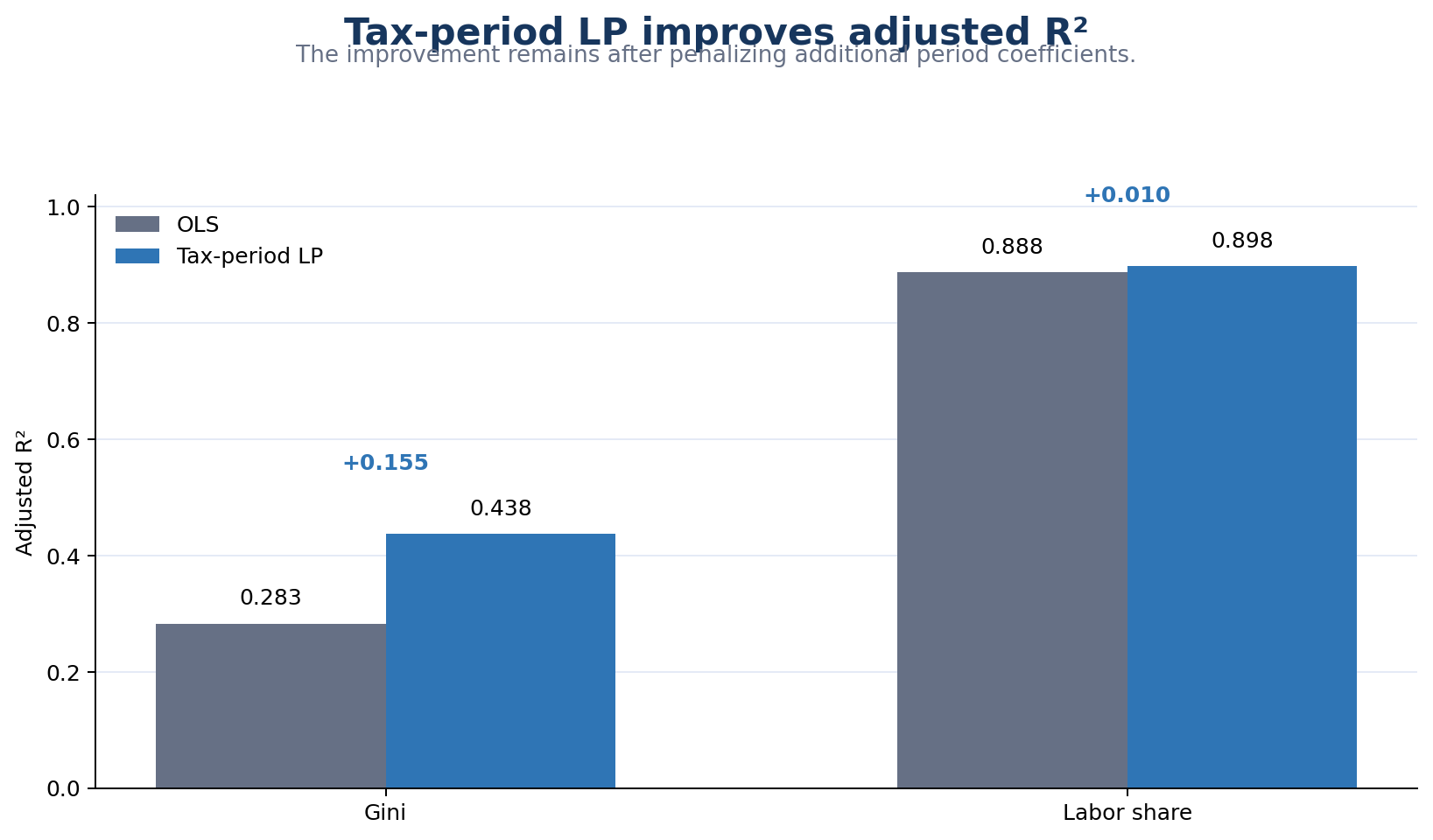
| Outcome | Model | Observations | R² | Adjusted R² | MAE |
|---|---|---|---|---|---|
| Gini | OLS | 62 | 0.307 | 0.283 | 1.567 |
| Gini | Tax-period LP | 62 | 0.521 | 0.438 | 0.959 |
| Labor share | OLS | 38 | 0.894 | 0.888 | 0.00833 |
| Labor share | Tax-period LP | 38 | 0.912 | 0.898 | 0.00652 |
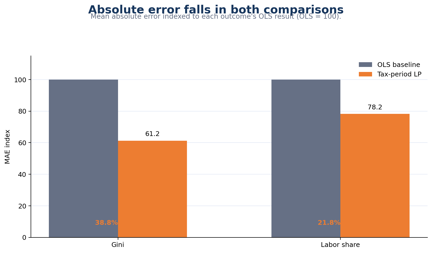
For Gini, the gain is substantial: adjusted R² improves by 0.155 and mean absolute error falls by 38.8%. For labor share, OLS already explains most of the variation, so LP produces a smaller adjusted-R² gain of 0.010 while reducing mean absolute error by 21.8%.
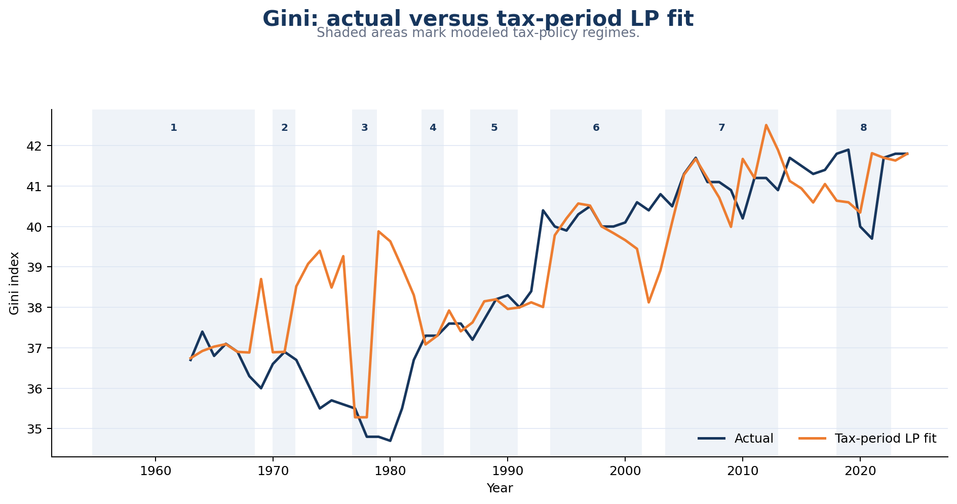
Gini: the average slope leaves history on the table
The OLS baseline estimates a positive average association between CP/GNP and Gini. The tax-period LP fit preserves a positive base relationship while allowing its strength to vary. One period—the 1976–1978 regime—lands exactly at the zero-slope boundary. Other periods range from roughly 24.9 to 77.8 Gini-index units per unit of the CP/GNP ratio.
That is more informative than declaring one eternal slope and going home early. It says the association is not equally strong in every policy window. It does not say which tax law caused what; history has more confounders than a family group chat.
| Regime | Start | End | Gini effective slope |
|---|---|---|---|
| 1 | 1954-08-16 | 1968-06-28 | 24.923 |
| 2 | 1969-12-30 | 1971-12-10 | 30.739 |
| 3 | 1976-10-04 | 1978-11-06 | 0.000 (binding) |
| 4 | 1982-09-03 | 1984-07-18 | 36.318 |
| 5 | 1986-10-22 | 1990-11-05 | 57.961 |
| 6 | 1993-08-10 | 2001-06-07 | 77.809 |
| 7 | 2003-05-28 | 2013-01-02 | 60.887 |
| 8 | 2017-12-22 | 2022-08-16 | 55.650 |
Labor share: a smaller gain can still matter
The labor-share baseline is already strong. Its OLS slope is negative (−1.207), and the LP period-effective slopes remain negative, ranging from about −1.00 to −1.24 across the four policy windows represented in the 1987–2024 sample.
Here LP is a refinement rather than a rescue. That distinction matters. A method worth trusting should be able to say “small improvement” without reaching for a fog machine.
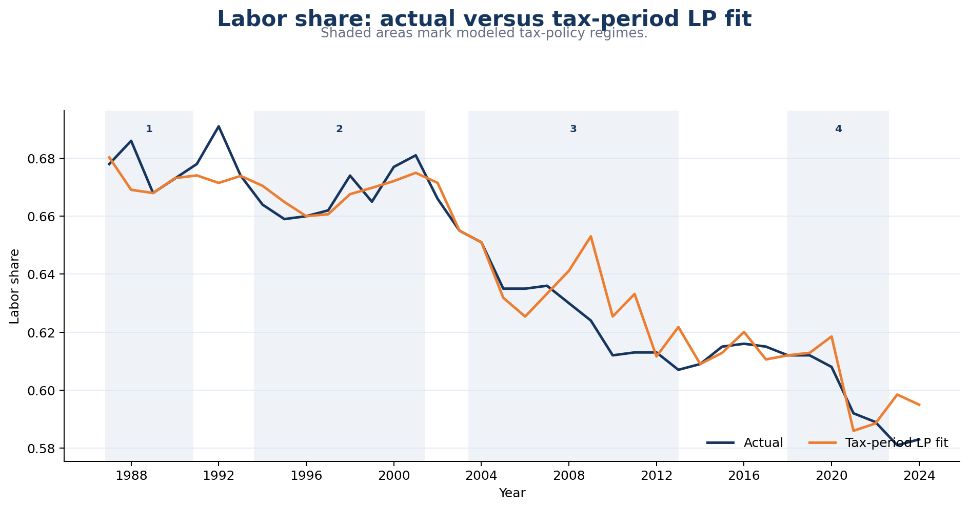
What improved—and what did not
The exercise supports a practical claim: LP regression can improve inspection of policy changes by exposing period-specific relationships that a single OLS coefficient averages away. The Gini result shows that the improvement can be large. The labor-share result shows that it need not be.
But this is still descriptive modeling. Tax-policy periods coincide with recessions, monetary changes, demographic shifts, trade shocks, technology, transfers, and many other forces. Annual frequency and same-date alignment simplify timing. Neither a higher adjusted R² nor a lower error establishes a causal tax effect. For causal claims, the next step would require a research design—credible counterfactuals, controls, timing assumptions, and robustness tests—not merely a more charming regression.
Reproduce the analysis
The complete RainbowStats slideshow contains both OLS baselines, the LP model summaries, coefficients, fitted values, residual diagnostics, shadow prices, and annotated actual-versus-fit charts.
Sources and definitions
The predictor uses Corporate Profits After Tax (CP) divided by Gross National Product (GNP). Outcomes are the World Bank's GINI Index for the United States and the BLS Private Nonfarm Business Sector: Labor Share, all accessed through FRED. The Stewart line refers to his concurrence in Jacobellis v. Ohio (1964). Calculations and graphics are reproduced from the linked RainbowStats analysis.