In the previous article, Four Measures of Money—and Why “Fed Liquidity” Is Not One Number, I separated four quantities that are frequently collapsed into the single word liquidity: M2, the Federal Reserve’s balance sheet, commercial-bank reserve balances, and a net-liquidity proxy that subtracts the overnight reverse-repurchase facility and the Treasury General Account from Federal Reserve assets.
That distinction leads naturally to a harder question.
Even if the Federal Reserve influences the aggregate supply of monetary liquidity, can it determine where that liquidity goes?
The answer is no. The Fed can change the policy rate, alter the size and composition of its balance sheet, and affect the quantity of reserve balances. It cannot instruct capital markets to finance another house rather than a semiconductor plant, a data center, a research program, or the federal deficit. Capital is allocated through a competitive process involving expected returns, risk, collateral, regulation, maturity, and the willingness of savers and intermediaries to supply financing.
This matters because housing is frequently treated as if it were the entire investment market. Mortgage rates are high, housing affordability is poor, and residential construction is weak. Those facts are real. But they do not establish that monetary policy is equally restrictive for every borrower and every investment category.
Since 2022, residential investment has competed with an extraordinary expansion in intellectual property, computing equipment, manufacturing structures, and federal financing needs. At the same time, the net-liquidity proxy has been broadly stable near $6 trillion. The result resembles a constrained capital-allocation problem: competing projects and borrowers are bidding for financing against a balance-sheet constraint that is no longer expanding rapidly.
The interest rate is the price that helps solve that allocation problem.
RainbowStats replication: Run the complete analysis in RainbowStats
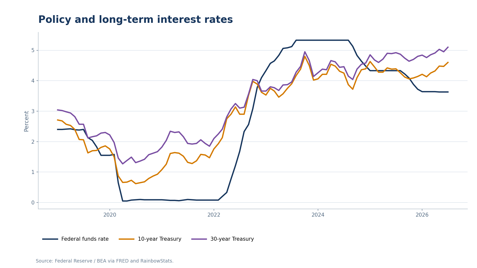
The Federal Reserve has substantial influence over the overnight federal funds rate. The 10- and 30-year Treasury yields are different. They incorporate the expected future path of short rates, expected inflation, the term premium, Treasury issuance, foreign demand, regulatory demand for safe assets, and the willingness of investors to hold duration.
That distinction is visible after 2022. The federal funds rate rose rapidly as the Fed responded to inflation. Long Treasury yields also rose, but they did not simply trace the policy rate. More recently, the federal funds rate declined while long yields remained comparatively elevated. By July 2026, the effective federal funds rate was approximately 3.6%, while the 10-year Treasury yield was approximately 4.6% and the 30-year yield was approximately 5.1%.
This is not what we would expect if the central bank mechanically controlled every interest rate. It is consistent with a market in which inflation expectations, term premiums, Treasury supply, and competing demands for long-term financing continue to matter even after the central bank begins easing the overnight rate.
Figure 1. Policy and long-term interest rates
Federal funds, 10-year Treasury, and 30-year Treasury yields since 2019.
The Fed sets an important price at the short end of the market. It does not allocate the resulting supply of credit across industries. Nor can it guarantee that a reduction in the overnight rate will be transmitted equally to mortgages, corporate bonds, construction loans, venture financing, or long-duration technology investment.
To see the allocation problem, begin with five broad categories of fixed investment:
Indexing real investment to the first quarter of 2019 produces a striking divergence. By the second quarter of 2026, real residential investment was approximately where it began. Real nonresidential structures were also close to their 2019 level after a powerful construction cycle and subsequent retreat. Equipment investment was about 24% above its 2019 level. Intellectual-property investment was about 67% higher. Real government investment was about 18% higher.
Figure 2. Real fixed investment, 2019 Q1 = 100
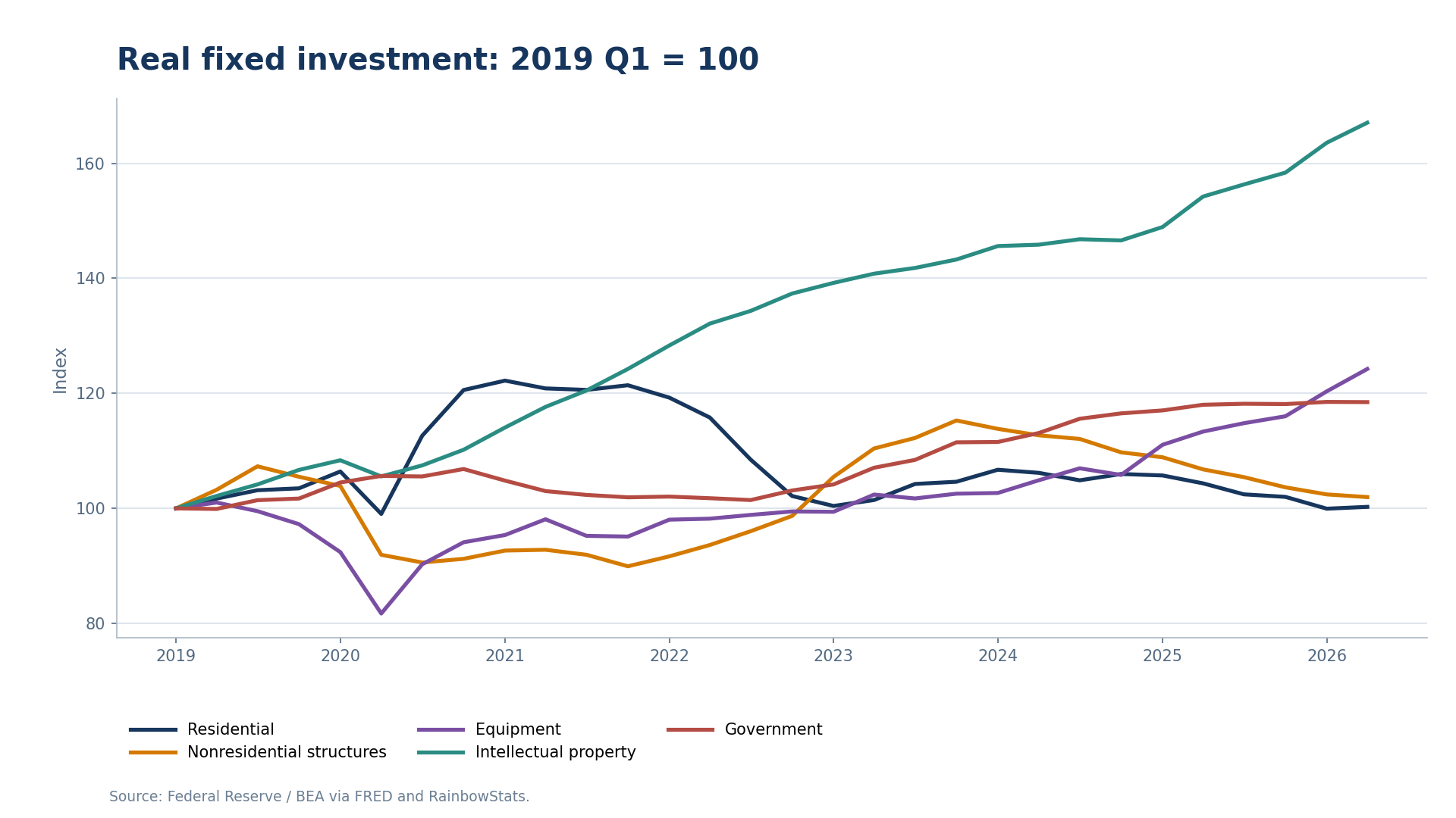
Residential, nonresidential structures, equipment, intellectual property, and government investment.
The divergence is even clearer in year-over-year growth rates. Housing weakened sharply when mortgage rates increased. Equipment and intellectual property did not follow the same path. Government investment also continued growing through much of the period.
The correct conclusion is not that interest rates are irrelevant. Housing is unusually sensitive to long-duration financing costs because the household purchase decision is tied directly to the monthly mortgage payment. The conclusion is that a single interest-rate environment can affect different investment categories very differently.
Housing competes for capital. It is not entitled to receive a fixed share of it.
Growth rates can be misleading if the underlying categories differ greatly in size. A small category can grow rapidly without absorbing much capital, while a large category can grow slowly and still account for an enormous financing flow.
The current-dollar shares therefore provide a necessary second perspective. Residential structures, nonresidential structures, equipment, intellectual property, and government investment together describe the broad fixed-investment market more completely than housing alone.
By 2026, equipment and intellectual-property products each represented roughly one-quarter of this combined fixed-investment measure. Government investment represented about one-sixth. Residential investment was important, but it was only one claimant among several.
Figure 3. Fixed-investment spending shares in current
dollars
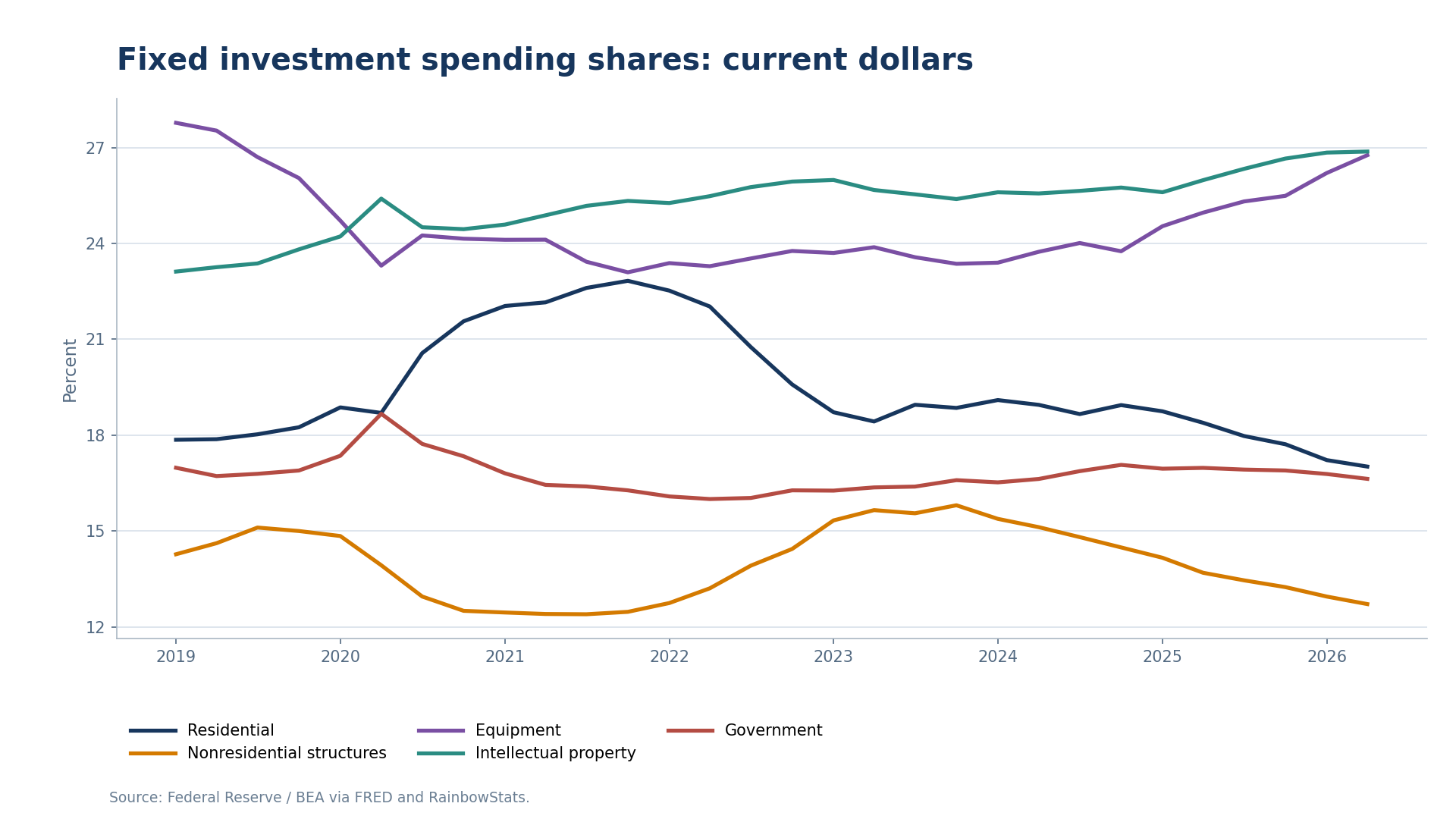
The composition of residential, business, intellectual-property, and government investment.
This is the first place where the usual housing narrative becomes incomplete. Higher mortgage rates can suppress housing while capital continues flowing toward equipment, software, research, factories, public infrastructure, and Treasury securities. Aggregate liquidity does not disappear merely because one sector cannot compete successfully at the prevailing price.
There is no official national-account series called “AI investment.” Any empirical proxy must therefore be described carefully. The RainbowStats analysis combines three current-dollar categories:
These categories are AI-sensitive, but they are not exclusively AI. Manufacturing structures include factories unrelated to artificial intelligence. Computers and peripherals have many uses. Research and development spans the entire economy. Conversely, the proxy omits portions of data-center construction, electric-power infrastructure, communications networks, and software that support AI deployment.
It is a broad directional proxy, not an accounting identity.
Even with that qualification, the change is dramatic. Real manufacturing-structure investment more than doubled from its 2019 level at its peak. Real investment in computers and peripherals approached three times its 2019 level by 2026. Real research-and-development investment rose by almost one-half.
Figure 4. Selected structures: real investment, 2019 Q1 =
100
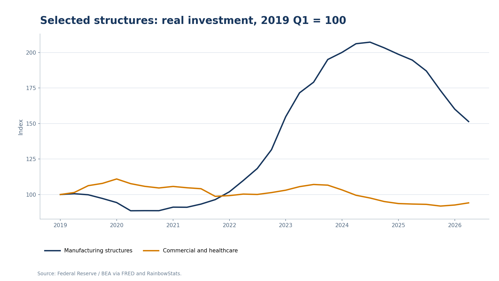
Manufacturing structures compared with commercial and healthcare structures.
Figure 5. AI-sensitive equipment and intellectual property,
2019 Q1 = 100
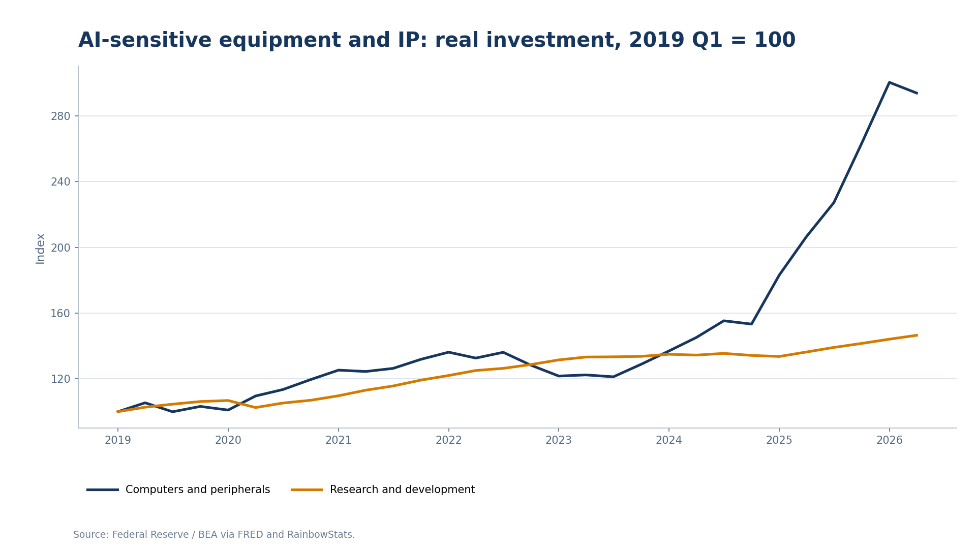
Computers and peripherals compared with research and development.
These are precisely the kinds of projects that may continue attracting capital when housing weakens. A corporation expecting a high return from computing capacity, automation, or research may be willing to finance a project at an interest rate that makes a marginal housing purchase unaffordable. The market does not ask which sector is politically popular. It compares expected returns, risks, and financing terms.
The original private-investment comparison omitted a very large participant: government.
Government affects the capital-allocation problem through two distinct channels, and they should not be confused.
First, gross government investment measures spending that creates public capital. It includes federal, state, and local investment in structures, equipment, and intellectual-property products. Real state and local investment has risen especially strongly in recent years, while federal real investment remains above its 2019 level.
Figure 6. Real federal and state-and-local government
investment
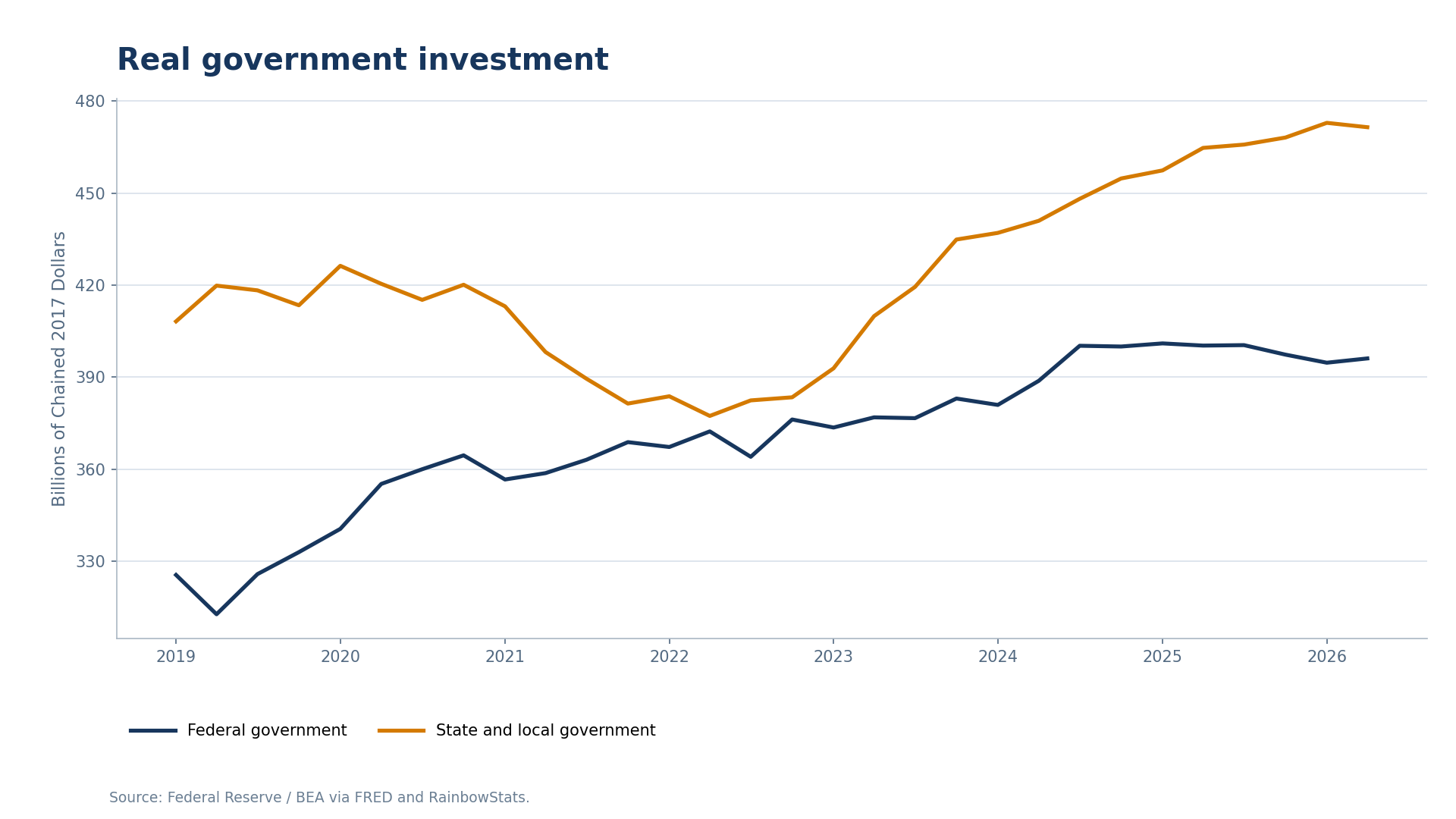
Billions of chained 2017 dollars.
Second, federal net borrowing represents a much broader financing requirement. The federal deficit does not finance only investment. It also reflects current expenditures, transfers, interest expense, and revenues. Nevertheless, the resulting borrowing must be absorbed by investors and intermediaries. Treasury securities therefore compete for balance-sheet capacity and investor portfolios even when the underlying federal expenditure is not classified as investment.
This distinction is crucial. Gross government investment belongs in the comparison of real capital formation. Federal net borrowing belongs in the comparison of financing demands placed on capital markets.
Government borrowing does not mechanically remove one dollar from private investment for every dollar borrowed. Foreign saving can enter the market. Private saving can increase. Banks and nonbanks can expand their balance sheets. Asset prices and interest rates can adjust. But when government financing needs rise while the supply of financing is constrained, the adjustment cannot be ignored. The price of capital must help reconcile demand with supply.
There is also an important asymmetry between government and private borrowers. A private investment normally must satisfy a return equation. Its expected return must compensate for its funding cost, risk, and use of scarce balance-sheet capacity. A project that cannot clear that hurdle is postponed, resized, or abandoned.
Government is not constrained by the same project-level return equation. It can borrow to finance public investment, current consumption, transfers, interest expense, or a politically chosen objective without demonstrating that the expenditure will earn a market return above the Treasury rate. Government still faces an intertemporal budget constraint, and rising interest expense can eventually constrain fiscal choices. But that is different from the contemporaneous return hurdle confronting a private borrower.
This makes government borrowing a special claim on the financing constraint. It does not have to win the same expected-return competition before entering the market.
The post-2022 period provides a useful test.
The net-liquidity proxy is defined as:
The measure is not a complete description of financial conditions. It omits bank capital, private credit creation, money-market intermediation, foreign capital, collateral constraints, and many other sources of financing. It is best interpreted as a balance-sheet proxy for liquidity supplied through the Federal Reserve system.
Within that definition, the post-2022 pattern is clear. Quarterly average net liquidity fell from approximately $6.6 trillion in early 2022 toward $6 trillion and then remained within a comparatively narrow range. It was about $5.9 trillion by July 2026.
Figure 7. Net-liquidity proxy since January
2022
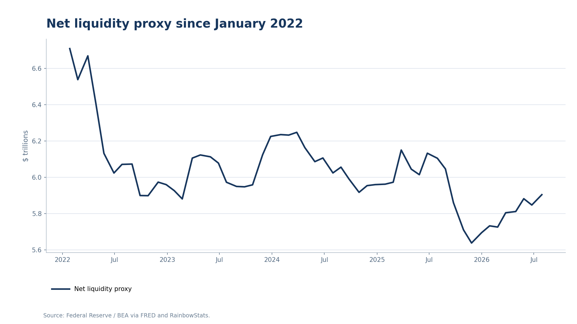
Federal Reserve assets less overnight reverse repos and the Treasury General Account.
Liquidity was not collapsing continuously. Nor was it expanding to accommodate every new demand. It was broadly constrained.
Meanwhile, the AI-sensitive investment proxy and federal net borrowing increased. Combining them creates a selected financing-demand measure. Dividing that annualized current-dollar flow by the quarterly average net-liquidity stock produces a financing-pressure proxy:
The numerator is a flow expressed at an annual rate. The denominator is a balance-sheet stock. Consequently, this is not a utilization ratio and should not be read as “the percentage of liquidity consumed.” It is a directional measure of financing demand relative to a constrained liquidity base.
The ratio rose from approximately 36% in early 2022 to around 51% by early 2023. It generally remained above 50% thereafter and temporarily exceeded 70% when federal net borrowing jumped in early 2026.
Figure 8. Selected private and federal financing
demand
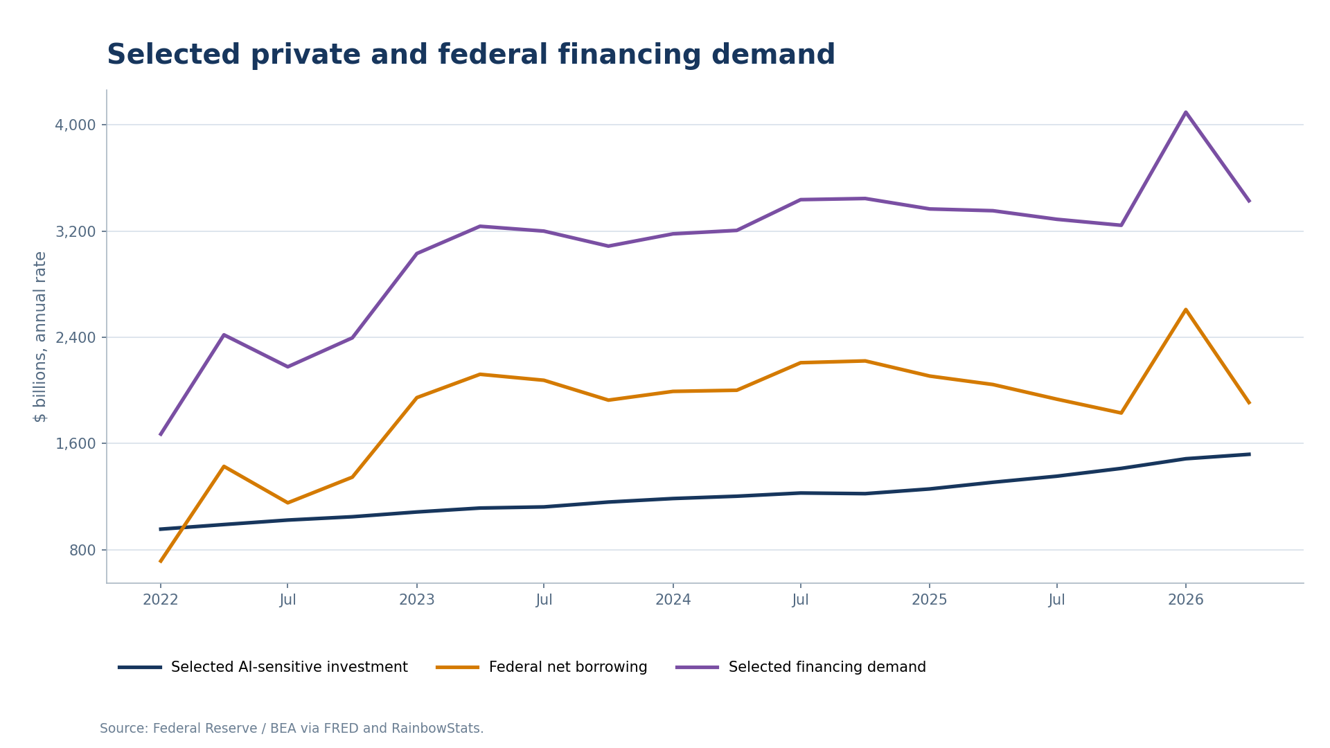
AI-sensitive investment, federal net borrowing, and their combined annualized flow.
Figure 9. Annualized financing demand relative to the
net-liquidity stock
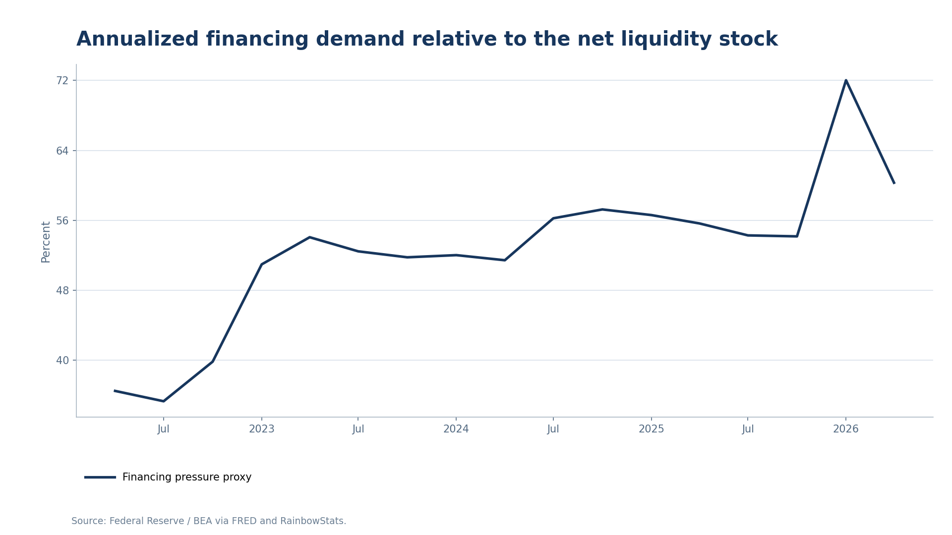
A directional financing-pressure proxy, not a utilization rate.
This is the heart of the argument. The relevant question is not simply whether the Fed created liquidity. It is whether the supply of financing expanded as quickly as the claims being placed upon it.
After 2022, the answer appears to be no.
The capital market can be viewed as a stylized constrained-optimization problem. Suppose private capital is allocated among projects indexed by . Each project has an expected risk-adjusted return , requires financing , and consumes some amount of intermediary balance-sheet capacity. Government borrowing represents an externally determined claim on available financing capacity .
A deliberately simplified representation is:
The private allocation is subject to:
The coefficients allow different investments to consume different amounts of scarce capital, collateral, or regulatory capacity. The Lagrange multiplier on the constraint, , is its shadow price. It measures the marginal value of relaxing the financing constraint.
Writing the constraint as makes the asymmetry explicit. Private projects are selected according to their expected risk-adjusted returns. Government borrowing enters outside that objective function. It reduces the financing capacity available to the private optimization problem without first having to demonstrate a comparable market return.
When financing capacity is abundant, is low. Many projects can be financed. When government borrowing and high-return private investment increase while remains relatively fixed, the constraint becomes more binding and rises.
Market interest rates, credit spreads, and required returns are observable—but imperfect—manifestations of that shadow price.
This is an analogy, not a literal structural model. Capital markets contain many constraints rather than one. Financing supply is endogenous. Borrowers differ in credit risk, collateral, duration, and access to markets. Some government expenditures can raise future productivity and expand , thereby crowding private investment in rather than out. Nevertheless, the framework captures an important reality: scarce balance-sheet capacity must be allocated, and its price rises when competing claims increase faster than financing capacity.
Housing can lose this competition without the Fed directing a single dollar away from it.
The empirical and theoretical arguments genuinely run in both directions.
The case against crowding out begins with the fact that financing capacity is not fixed. Banks create credit. Higher rates can attract additional saving. Foreign investors can purchase Treasury securities. Treasuries provide safe assets and collateral that support market intermediation. Public infrastructure, research, and education can increase private productivity and encourage additional investment. If government spending expands the economy’s productive capacity, it may crowd private investment in rather than out.
Monetary conditions also matter. During periods of excess reserves and aggressive central-bank accommodation, government borrowing can increase without producing an obvious rise in long rates. The enormous federal financing requirement during the pandemic coincided initially with exceptionally low Treasury yields because monetary accommodation and risk aversion overwhelmed the normal price response.
The case for crowding out begins with the observation that real-world financing capacity is never infinitely elastic. Banks face capital and liquidity requirements. Dealers have finite balance sheets. Investors have duration limits and portfolio mandates. Foreign demand is variable rather than guaranteed. When Treasury issuance, high-return corporate investment, and household borrowing all rise together, some combination of interest rates, credit spreads, asset prices, and quantities must adjust.
The government’s exemption from the private return equation strengthens this side of the argument. A marginal private project disappears when its expected return falls below its financing cost. A federal borrowing requirement does not disappear merely because the associated expenditure offers no measurable market return. The Treasury continues financing the authorized deficit, and the price adjustment is transmitted to the borrowers that do face return constraints.
The post-2022 evidence cannot settle this debate universally. It does show a period in which the net-liquidity proxy remained broadly stable, selected financing demands increased, long yields rose, and residential investment weakened. That is the pattern we would expect if the financing constraint had become more binding.
The first regression relates the average of the quarterly 10- and 30-year Treasury yields to the financing-pressure proxy over the post-2022 sample.
The level regression produces:
The sign is consistent with the hypothesis. A one-percentage-point increase in the financing-pressure proxy is associated with approximately 4.4 basis points in the average long Treasury yield within this short sample.
Figure 10. Long Treasury yields and financing
pressure
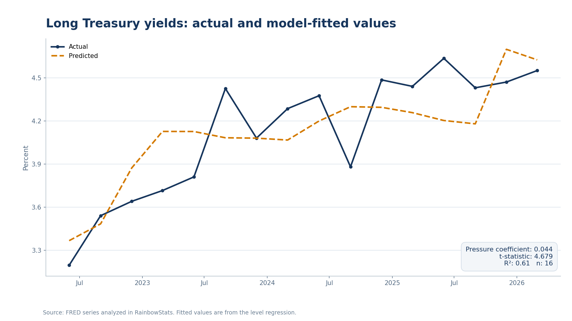
Regression of the average 10- and 30-year Treasury yield on the financing-pressure proxy.
An R² of 0.61 is notable for such a simple relationship, but it is not a causal estimate. Both variables can respond to inflation, fiscal policy, expected Fed policy, and the business cycle. The sample begins during an extraordinary monetary tightening and contains only sixteen quarterly observations.
The regression nevertheless supports the descriptive argument: higher financing demand relative to a stable liquidity proxy has coincided with a higher shadow price for long-duration capital.
The second regression relates real residential investment to the same financing-pressure proxy.
The level regression produces:
The negative sign is again consistent with crowding out. Higher financing pressure is associated with lower real residential investment.
Figure 11. Real residential investment and financing
pressure
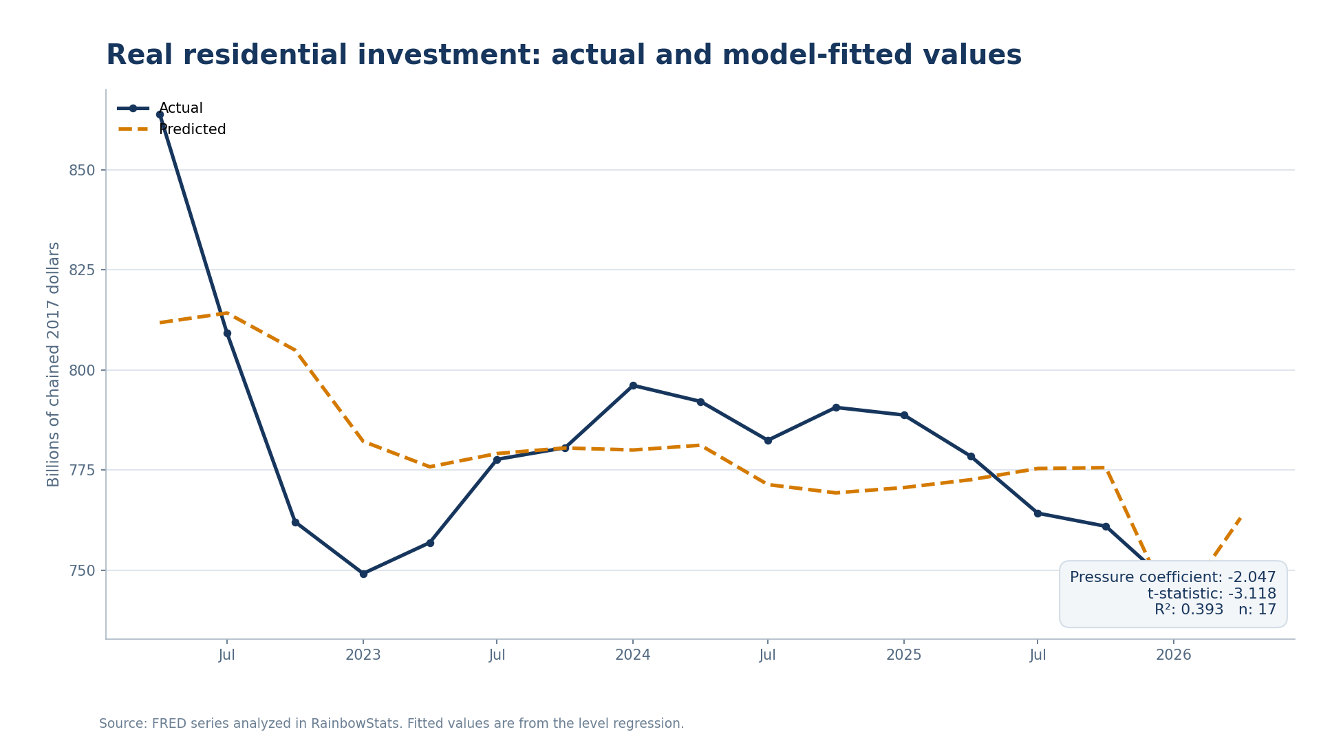
Regression of real residential investment on the financing-pressure proxy.
This does not mean federal borrowing or AI investment directly “caused” a particular housing project to disappear. The mechanism is mediated through rates, credit standards, land prices, construction costs, household income, and expected returns. But it does show that housing weakened during a period in which other financing demands rose against a comparatively stable liquidity stock.
That is a more complete explanation than saying simply that “the Fed made rates restrictive.” The Fed helped establish the interest-rate environment. The market then allocated capital among competing uses.
The evidence becomes weaker when the regressions are estimated in first differences.
For quarterly changes in the long Treasury yield against changes in financing pressure, the R² is approximately 0.01. For residential-investment growth against changes in financing pressure, the R² is approximately 0.06. Neither result provides persuasive quarter-to-quarter evidence.
That weakness should not be hidden. Level regressions over a short trending sample can produce strong associations even when the underlying causal relationship is more complicated. Interest rates may move before investment spending is recorded. Borrowing plans can be anticipated. Fed policy and inflation expectations can dominate quarterly changes. Residential investment can respond with a lag.
The honest conclusion is therefore narrower:
The post-2022 data display a pattern consistent with crowding out under a constrained liquidity stock. They do not, by themselves, prove a structural causal effect.
That is still an important result. A model does not need to explain every quarterly movement to improve our understanding of the broader allocation problem.
Public discussion often asks whether monetary policy is “restrictive” as though every sector confronts the same constraint. The investment data show why that language can mislead.
Housing is weak. Intellectual-property investment is strong. Computing investment has surged. Manufacturing construction experienced a historic expansion. Government investment is above its 2019 level. Federal borrowing remains large. Corporate profits can remain high while mortgage affordability deteriorates because the same interest rate is applied to projects with very different expected returns and financing structures.
The Fed can supply reserves and influence the policy rate. It cannot compel a bank to make a construction loan, require an investor to buy a mortgage-backed security, or order a corporation to abandon a high-return computing project in favor of residential development.
Nor can the Fed eliminate the fiscal financing requirement. Treasury securities must be absorbed by the market. When the Treasury, AI-sensitive businesses, and households all seek long-duration financing, prices and quantities adjust. High-return private projects may continue because they can clear the higher hurdle rate. The government continues borrowing because it is not subject to that private return equation. Marginal, rate-sensitive projects are postponed or canceled.
This is not necessarily a market failure. It is the allocation mechanism working through a higher shadow price.
The previous article showed why money and liquidity cannot be reduced to one number. This analysis adds the next step: even aggregate liquidity does not tell us where capital will go.
Since 2022, the Federal Reserve’s net-liquidity proxy has remained broadly stable near $6 trillion. Over the same period, selected AI-sensitive investment and federal borrowing increased the financing demands placed on capital markets. Long Treasury yields rose, while real residential investment weakened.
The level regressions are consistent with a crowding-out interpretation. The first-difference tests are not strong enough to establish causality. The linear-programming analogy therefore should be understood as an organizing framework: when competing claims rise against constrained financing capacity, the shadow price of capital rises and lower-return or more rate-sensitive projects lose access at the margin.
Government occupies a distinctive position in that framework. Private projects must clear the market’s return hurdle. Government borrowing enters the constraint without being selected by the same equation. Public investment may ultimately expand productive capacity, but the immediate financing claim still has to be absorbed.
The Fed supplies liquidity. It influences the price of short-term money. But it does not decide whether the next dollar finances a home, a semiconductor plant, a research laboratory, a data center, public infrastructure, or the federal government.
Markets make that decision.
The analysis uses Federal Reserve, Federal Reserve Bank of New York, U.S. Treasury-rate, and Bureau of Economic Analysis series distributed through FRED and analyzed in RainbowStats.
The net-liquidity proxy is Federal Reserve total assets
(WALCL) less overnight reverse repurchase agreements
(RRPONTSYD) and the Treasury General Account
(WDTGAL). The source series have different native
frequencies and units; RainbowStats aligns their units before monthly
and quarterly aggregation.
The AI-sensitive investment proxy combines current-dollar
manufacturing structures (C307RC1Q027SBEA), computers and
peripherals (B935RC1Q027SBEA), and research and development
(Y006RC1Q027SBEA). Federal net borrowing is
AD02RC1Q027SBEA. Real residential investment is
PRFIC1. Long rates are the 10-year (GS10) and
30-year (GS30) constant-maturity Treasury yields.
The sample ends July 31, 2026. The regressions are descriptive and should not be interpreted as identified causal estimates.
The accompanying publication package contains tidy CSV data for every figure, actual-versus-fitted regression series, a regression-summary table, the exact RainbowStats script, and the raw structured RainbowStats chart and regression results.