Instrument Hacking
How searching for the “best” instrumental variable can manufacture statistical significance and pull IV estimates back toward the biased OLS result.
Instrumental variables are supposed to rescue a causal estimate when an explanatory variable is endogenous. But what happens when a researcher has several plausible instruments, estimates every version of the model, and reports the one with the strongest first stage or the most attractive second-stage t statistic?
Michael P. Keane, Timothy Neal, and Patrick Vu call this instrument hacking. Their result is both surprising and uncomfortable: even when every candidate instrument is valid and reasonably strong, selecting among them can bias the reported IV estimate toward the OLS estimand and badly distort conventional t tests. The practice need not be dishonest. A researcher may sincerely believe that choosing the largest first-stage F statistic is prudent. The selection step itself is the problem.
The experiment
The paper studies a single-equation IV model with one endogenous regressor:
The illustrative design sets the true effect β to zero and endogeneity ρ to 0.5, so the OLS estimand is positive even though the causal effect is not. There are ten equally strong Bernoulli instruments, each with assignment probability 0.5 and π = √0.3. The sample contains 350 observations. Each just-identified specification has a true first-stage F statistic of about 28.4—well above the familiar rule-of-thumb weak-instrument threshold.
The researcher observes K candidate instruments and reports one just-identified regression:
- Second-stage hacking: select the instrument producing the largest absolute t statistic, max |t|.
- First-stage hacking: select the instrument producing the largest sample first-stage F statistic.
RainbowStats repeats the experiment 10,000 times for K = 1, 3, and 10. The original paper uses 100,000 replications in Figure 1, so small Monte Carlo differences are expected.
RainbowStats results
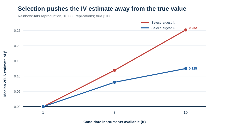
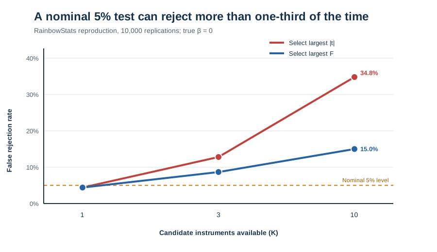
Second-stage selection: choose the largest |t|
| K | Median β̂ | P < 0.05 | Positive rejections | Median F |
|---|---|---|---|---|
| 1 | -0.000 | 4.4% | 96.6% | 28.349 |
| 3 | 0.119 | 12.8% | 96.8% | 29.578 |
| 10 | 0.252 | 34.8% | 96.4% | 33.989 |
First-stage selection: choose the largest F
| K | Median β̂ | P < 0.05 | Positive rejections | Median F |
|---|---|---|---|---|
| 1 | -0.000 | 4.4% | 96.6% | 28.349 |
| 3 | 0.080 | 8.7% | 99.3% | 38.123 |
| 10 | 0.125 | 15.0% | 99.9% | 47.419 |
Does RainbowStats reproduce the paper?
Yes. The principal results are nearly identical despite using one-tenth as many replications.
| Selection | K | Paper median β̂ | RainbowStats | Paper P < 0.05 | RainbowStats |
|---|---|---|---|---|---|
| Largest |t| | 1 | 0.00 | -0.000 | 4.4% | 4.4% |
| Largest |t| | 3 | 0.12 | 0.119 | 12.4% | 12.8% |
| Largest |t| | 10 | 0.25 | 0.252 | 35.7% | 34.8% |
| Largest F | 1 | 0.00 | -0.000 | 4.4% | 4.4% |
| Largest F | 3 | 0.08 | 0.080 | 8.6% | 8.7% |
| Largest F | 10 | 0.13 | 0.125 | 15.4% | 15.0% |
Why does this happen?
The mechanism is not simply “try enough regressions and something will be significant.” IV adds a more specific distortion that Keane and Neal call power asymmetry. In finite samples, the 2SLS estimate and its standard error are related. Standard errors tend to be smaller when the IV estimate lies closer to the biased OLS estimand.
Selecting the largest |t| therefore favors a combination of a convenient coefficient and a convenient standard error. Selecting the largest first-stage F statistic sounds safer, but it still conditions on a sample statistic that is related to the reported IV result. As K grows, the winning specification becomes increasingly exceptional. The median estimate moves toward 0.5, the OLS estimand in this design, even though the true β remains zero.
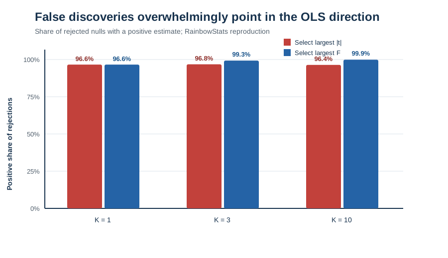
Notice the direction of the false discoveries. With ten instruments, 96.4% of second-stage false rejections and 99.9% of first-stage false rejections are positive. Random noise alone would not produce such one-sided errors. The selection mechanism is pulling results toward the direction of the endogeneity bias.
Strong instruments do not solve a selection problem
The experiment begins with instruments whose true F statistic is approximately 28.4. The problem is not that the researcher started with a collection of obviously weak instruments. Indeed, choosing the largest sample F pushes the median reported F to 47.4 when ten candidates are available. The reported first stage looks stronger while the causal estimate becomes less trustworthy.
This is not an argument against instrumental variables
The lesson is not that IV is useless. It is that research design must come before result selection. A credible instrument needs a substantive case for relevance and exclusion. If several instruments are available, the full candidate set and the selection process should be disclosed. Researchers should not treat the specification with the most appealing t statistic—or even the largest observed F—as though it had been chosen in advance.
Keane, Neal, and Vu recommend avoiding instrument selection and using all available instruments with robust estimation and inference. Under homoskedasticity they emphasize LIML with conditional likelihood-ratio inference; under heteroskedasticity they discuss continuously updated GMM with weak-instrument-robust inference. Their broader message is that conventional 2SLS t tests are especially vulnerable after instrument selection.
Reproduce it in RainbowStats
The complete experiment takes two commands:
H=INSTRUMENT_HACKING(10000)
SLIDESHOW(H)
The underlying simulated estimates can also be extracted for further analysis:
B1=EXTRACT(H,"beta_second_k1")
B3=EXTRACT(H,"beta_second_k3")
B10=EXTRACT(H,"beta_second_k10")

F1=EXTRACT(H,"beta_first_k1")
F3=EXTRACT(H,"beta_first_k3")
F10=EXTRACT(H,"beta_first_k10")A warning for applied IV work
Before accepting an instrumental-variable result, ask four questions: Why is the regressor endogenous? Why is the instrument relevant? Why should the instrument satisfy the exclusion restriction? And how many alternative instruments or specifications were examined before this result was reported?
RainbowStats now includes IV_REGRESSION to estimate and inspect first- and second-stage results.
The tool makes the calculations transparent, but no statistical command can supply the missing economic argument
for instrument validity. That burden remains with the researcher.
Source
- Michael P. Keane, Timothy Neal, and Patrick Vu, “Instrument Hacking,” NBER Working Paper No. 35633, August 2026. Paper and data appendix at NBER.