German Reunification: When Politics Changed the Quantity of Money
Introduction
In March 2025, I wrote about the economic consequences of German reunification.
The idea was deliberately simple. I imagined two economies—Country A and Country B. Country A had a stable currency and functioning market economy. Country B had a very different economic system, lower productivity, and a currency whose official value did not necessarily represent the value at which the market would have exchanged it.
Now merge the countries.
What happens if political authorities choose a currency-conversion rate substantially more generous than the rate implied by economic fundamentals?
At the time, I treated it principally as an equation problem. Since then, RainbowStats has developed considerably. We now have the historical German interest-rate and foreign-exchange series, event markers, time-series transformations and multivariate transfer-function analysis necessary to revisit the question using actual data.
So I went back to 1990.
The result is more interesting than my original argument.
Two countries, two currencies
The Berlin Wall fell on November 9, 1989. German political events then moved extraordinarily quickly. Monetary, economic and social union took effect on July 1, 1990, extending the Deutsche Mark and the Bundesbank's monetary-policy responsibility to East Germany. Political reunification followed on October 3.
It is tempting to remember the currency conversion simply as “one East German Mark became one Deutsche Mark.” The actual arrangement was more complicated. Wages, salaries, pensions, rents and other recurring payments were converted at 1:1. Most other claims and liabilities were generally converted at 2:1, with specified amounts of personal savings eligible for conversion at 1:1.
That distinction matters. This was not merely changing the symbol printed on a banknote. Monetary claims denominated in one currency were being transformed into claims denominated in one of the world's strongest currencies.
The Country A/Country B experiment
Let Country A's existing money stock be M_A and let Country B have monetary claims M_B.
Suppose the economically appropriate conversion value of Country B's currency is v units of Country A's currency. The hypothetical combined money stock at that valuation is:
M* = M_A + v M_B
Now suppose political authorities instead choose a more favorable conversion factor c. The post-conversion money stock becomes:
M_1 = M_A + c M_B
The difference is:
ΔM = (c − v) M_B
If c > v, the political conversion recognizes more Country-A-denominated monetary claims than our assumed economic valuation would have produced. That does not tell us exactly what happens next, but it tells us that something has changed.
The monetary discontinuity
The Bundesbank's historical accounts make clear that the monetary change was large. About 25 million accounts had to be converted. East German citizens had roughly 180 billion East German Marks in savings and giro accounts and, following conversion, held roughly DM120 billion.
More broadly, the conversion increased Deutsche-Mark M3 by approximately DM180 billion—almost 15 percent of the existing West German M3 money stock.
This was not a rounding error. It was an enormous monetary event.
| German monetary union | Magnitude |
|---|---|
| Accounts converted | ~25 million |
| East German savings/giro balances before conversion | ~180bn East German Marks |
| DM balances held by citizens after conversion | ~DM120bn |
| Increase in DM M3 associated with conversion | ~DM180bn |
| Increase relative to West German M3 | Almost 15% |
Start with the quantity equation
The natural starting point is MV = PY, where M is money, V velocity, P the price level and Y real output. In approximate growth-rate form:
Δm + Δv = Δp + Δy
A simplistic interpretation would say that a large increase in money must produce a similarly large immediate increase in prices. But everything else was emphatically not constant. East Germany was changing economic systems. Money demand, access to goods, portfolio preferences, banking, fiscal transfers, investment, production and expectations all changed.
Critically, monetary policy changed too.
The absence of an immediate inflation increase matching the monetary jump does not invalidate monetary economics. It tells us that adjustment occurred through more variables than CPI alone.
The price of money
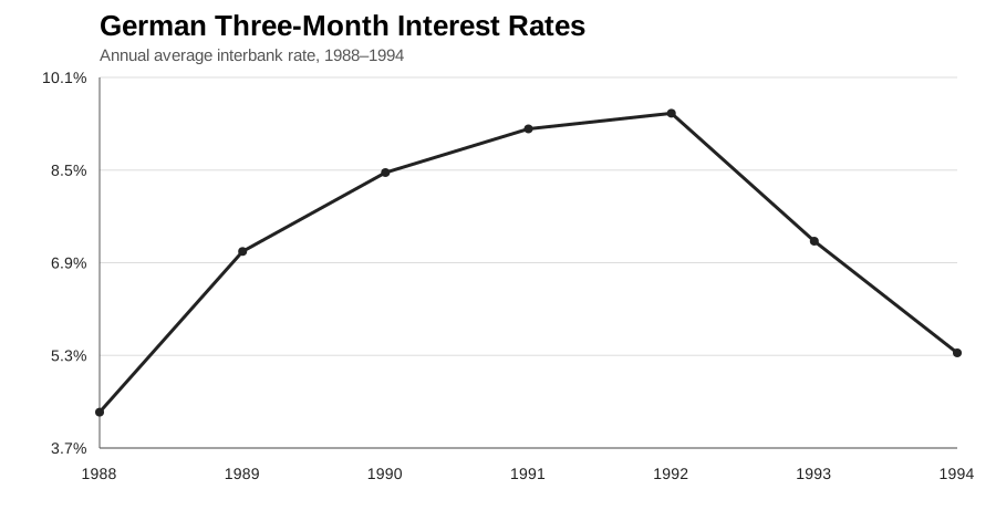
RainbowStats retrieves the German three-month interbank rate around reunification. Annual averages rose from about 4.33 percent in 1988 to 7.12 percent in 1989, 8.49 percent in 1990, 9.25 percent in 1991 and 9.52 percent in 1992 before declining.
The monthly chronology is even more revealing. The three-month rate was 5.70 percent in January 1989. By late 1989 it was above 8 percent. It remained above 8 percent around monetary union and ultimately approached 10 percent in 1992.
This chronology matters. We cannot say that monetary union occurred on July 1 and therefore rates suddenly jumped. German monetary tightening was already underway. Reunification arrived in the middle of that tightening cycle and added an enormous monetary and fiscal complication.
The price of short-term money became exceptionally high.
| Year | German 3-month interbank rate |
|---|---|
| 1988 | 4.33% |
| 1989 | 7.12% |
| 1990 | 8.49% |
| 1991 | 9.25% |
| 1992 | 9.52% |
| 1993 | 7.30% |
| 1994 | 5.36% |
Mark the events, not just the years
Markets react to information before a policy becomes legally effective. That is why the RainbowStats replication marks the fall of the Berlin Wall, the February 1990 currency-union announcement, the May State Treaty, July 1 monetary union, October 3 political reunification, and the later 1992 ERM crisis.
Looking only at October 3 would miss much of the economic experiment. Markets discount expectations.
Then something surprising happened to the Deutsche Mark
If our model stopped at ΔM > 0, we might expect the Deutsche Mark to weaken. The historical record is not that simple.
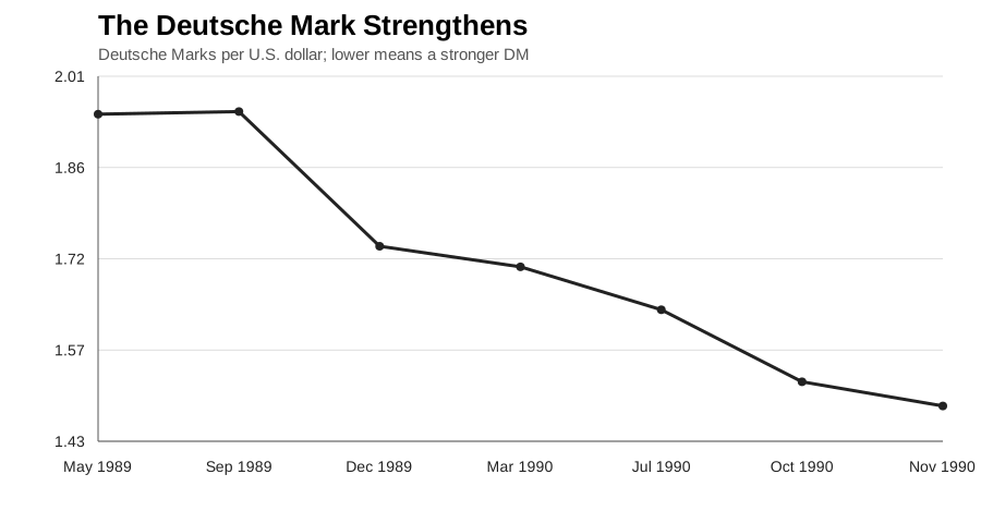
The FRED exchange-rate series is quoted as Deutsche Marks per U.S. dollar. A falling number therefore means a stronger Deutsche Mark. The quote fell substantially during the initial reunification period, from roughly 1.95 DM per dollar around September 1989 to roughly 1.49 by November 1990.
The Deutsche Mark appreciated.
Our original one-variable model was already incomplete. We had monetary expansion, but we also had high German interest rates, changing expectations and international capital flows.
| Month | DM per U.S. dollar |
|---|---|
| May 1989 | 1.9461 |
| Sep. 1989 | 1.9502 |
| Dec. 1989 | 1.7378 |
| Mar. 1990 | 1.7053 |
| Jul. 1990 | 1.6375 |
| Oct. 1990 | 1.5238 |
| Nov. 1990 | 1.4857 |
Add capital markets to the equation
Suppose German assets yield i_DE while foreign assets yield i*. International investors also care about expected exchange-rate changes and risk. Schematically:
K = f(i_DE − i*, E[ΔS], ρ)
Higher German interest rates, all else equal, make Deutsche-Mark assets relatively more attractive. A monetary expansion can therefore coexist with restrictive monetary policy, capital inflows and a strong currency.
This does not prove that high German rates caused the entire appreciation of the Deutsche Mark. Foreign-exchange markets are too complicated for that claim. It does show why “more money therefore weaker currency” is not an adequate model. The central bank is part of the system.
So we tested it
A persuasive chart can be dangerous. Two variables moving together can create a compelling narrative even when the statistical relationship is weak.
We therefore transformed the financial variables and used RainbowStats' multivariate transfer-function framework over the concentrated 1989–1992 reunification window. Instead of assuming that today's interest-rate movement must explain today's financial-market movement, the model allows relationships to work through time while modeling the remaining time-series structure.
The working RainbowStats specification uses LOGDIFF for the exchange rate, DIFF for short and long rates, and MVTransfer_Function with six lags and twelve regressions.
fxchange=LOGDIFF(fx)
ratechange=DIFF(rate)
bondchange=DIFF(bond)
data=LIST(fxchange,ratechange,bondchange)
tfFX=MVTransfer_Function(data,6,12)
The econometric result
The tighter reunification-period model produced an R² of 0.440, an adjusted R² of 0.378, an F-statistic of 9.689 and a Durbin-Watson statistic of 1.977. The selected changes in the German 10-year yield at lags three, four and five had coefficients of approximately −0.608, −0.923 and −0.565, with t-statistics of approximately −3.62, −4.67 and −3.00.
There is meaningful dynamic structure in the reunification window. The effects selected by the model are concentrated several months later rather than contemporaneously.
But the model does not establish that currency conversion caused every subsequent rate increase. It does not establish that Bundesbank tightening caused all Deutsche Mark appreciation. And it does not establish that reunification alone caused Europe's later monetary problems.
That restraint is important. Econometrics should test a story, not decorate a conclusion.
| Statistic | RainbowStats result |
|---|---|
| Observations | 41 |
| R² | 0.440 |
| Adjusted R² | 0.378 |
| F-statistic | 9.689 |
| Durbin-Watson | 1.977 |
| Standard error | 0.065 |
| AIC | −220.439 |
| BIC | −213.585 |
| Change in German 10-year yield | Beta | Std. error | t-stat |
|---|---|---|---|
| Lag 3 | −0.608 | 0.168 | −3.618 |
| Lag 4 | −0.923 | 0.198 | −4.666 |
| Lag 5 | −0.565 | 0.189 | −2.996 |
Where did the money go?
If conversion expanded M3 by almost 15 percent, why wasn't there an immediate 15 percent inflation shock?
Because money is not mechanically translated into CPI. In MV = PY, every variable can move. Money demand in East Germany could rise after access to a stable currency. Velocity could change. Real activity and imports could change. Asset prices, interest rates, capital flows and credit conditions could all adjust.
The correct lesson is not “M rises 10 percent, therefore P rises 10 percent.” The correct lesson is that MV = PY must still balance, and the economy has many ways of getting there.
The experiment escaped Germany
Germany did not operate in isolation. European currencies were linked through the European Monetary System and its Exchange Rate Mechanism.
In simplified form, interest parity can be written:
i_foreign ≈ i_DE + E(ΔS/S) + ρ
If policymakers simultaneously promise to keep the exchange rate within a narrow band, large and persistent interest-rate differentials become difficult to sustain. Capital moves. The lower-yielding country then faces choices: raise rates, intervene, devalue, or leave the arrangement.
By 1992 those tensions had become a European monetary crisis. Reunification was not the sole cause, but German monetary conditions were no longer merely a German matter.
What did the experiment establish?
The evidence is strongest when we separate observation from interpretation.
German monetary union produced a documented, large increase in Deutsche-Mark monetary claims. German short-term rates became exceptionally high. The Deutsche Mark initially strengthened. The RainbowStats transfer-function analysis finds meaningful dynamic structure in the rate system during the concentrated reunification window.
What it does not provide is a one-variable causal explanation for every movement in rates, foreign exchange or the later ERM crisis.
The data changed the story. That is a feature, not a problem.
A monetary experiment is not a trivial exercise
My original Country A/Country B equation was:
ΔM = (c − v) M_B
The real economy required something closer to:
ΔM → {P, Y, V, i, FX, Credit, Capital Flows}
All of those variables can participate in restoring equilibrium.
A government can legislate the denomination of a monetary claim. It can determine a conversion ratio. A central bank can create reserves. But none of those actions instantly creates factories, energy, housing, skilled workers, technology or productive capital.
Nominal claims are not the same thing as real resources.
Eventually they meet in markets, and markets have prices.
Thirty-six years later
German reunification was an extraordinary political achievement. Nothing in this analysis changes that, and showing that monetary union had economic costs does not decide whether those costs were justified.
What the episode gives us is something unusually valuable: a natural experiment.
We know when the announcements occurred. We know when monetary union occurred. We know approximately how much the money stock changed. We know what happened to German short and long rates. We know what happened to the Deutsche Mark. Today we can put those observations into an econometric model rather than merely tell a story about them.
The result is not that my original Country A/Country B equation was wrong. It was incomplete.
When a monetary imbalance is introduced, there is no rule saying the cost must appear where we expect it. It may appear in consumer prices, interest rates, currencies, asset markets, credit, or cross-border capital flows. Sometimes several adjust at once.
The absence of an immediate inflation crisis therefore does not establish that a monetary experiment was costless. It tells us to look at the rest of the equation.
This time, instead of Country A and Country B, we had the data.