The Wealth of Nations—Redux
Adam Smith began with productive labor. My question is modern: when we stop wasting human talent, does productivity become wealth—and does compounded wealth create still more opportunity?
Steven Durlauf’s New York Times essay, “Three Ways Trump Is Strangling Economic Growth,” stopped me at one claim: opening occupations to women and Black Americans may have produced between 20% and 40% of U.S. growth in market output per person from 1960 through 2010. I spent a career in markets, where an attractive story is never enough. RainbowStats is an econometric site. I wanted to see whether the public data could support the argument—or knock it down.
Durlauf is a University of Chicago economist whose work bridges microeconomics, macroeconomics, inequality and growth. The evidence he invokes also carries a strong Chicago pedigree. Chang-Tai Hsieh and Erik Hurst of Chicago Booth, together with Charles Jones and Peter Klenow of Stanford, asked how much American growth arose when women and Black Americans gained access to occupations that had once been dominated by white men. Their answer was large: across specifications, improved allocation of talent accounted for roughly 20% to 40% of growth in market output per person between 1960 and 2010.
The 20%–40% figure does not mean that one statute, one university office or every program labeled “DEI” produced that much growth. It comes from a structural model of occupational choice. The question underneath it is simpler: how much wealth does a nation sacrifice when people cannot follow their comparative advantage?
Today we mine the human intellect
My memory of Adam Smith was close, but not quite right. Nature supplies the raw material of wealth: the produce of the land and the resources beneath it. Labor adds value by transforming those resources. Smith put it more directly: “Labour was the first price, the original purchase-money that was paid for all things.” A nation’s abundance then depends on the skill, dexterity and judgment with which that labor is applied.
Coal or iron must be discovered, extracted and put to productive use. Human ability must be discovered, educated and matched to useful work. Unlike a mineral deposit, intellect grows when it is used. Education, experience and opportunity enlarge it. When a capable person is blocked from becoming a physician, scientist, engineer, teacher or entrepreneur, the economy leaves part of its richest resource underground.
The idea sounds obvious: unrestricted labor produces greater wealth. But “unrestricted” needs care. I do not mean a labor market without safety rules, contracts or standards. I mean labor freed from restrictions unrelated to ability. Nor does adding workers automatically raise productivity or household wealth. The stronger proposition is that better access improves matching, better matching raises output per hour, and some of that added income compounds into wealth. That accumulated wealth can then finance the next person’s education, business or opportunity.
The economic equation
The mechanism begins with growth accounting. Let (Y) denote real output, (P) population, (H) total hours, (E) employment and (L) the labor force. Then output per person can be written as:
Opportunity can operate on more than one term. When barriers fall, people previously discouraged from market work can enter the labor force, raising (L/P). If those people enter occupations that better match their skills, output per hour (Y/H) can rise. Improved job finding can raise (E/L), while movements between part-time and full-time work affect (H/E). The Hsieh–Hurst–Jones–Klenow result is principally about the first and second channels: more people participate, and talent is allocated more productively across occupations.
This is why labor-market slack, including U-6, is not the centerpiece of my presentation. U-6 is useful for diagnosing the business cycle. It measures unemployment, marginal attachment and involuntary part-time work, so it contains information about (E/L) and (H/E). But it begins only in 1994, is dominated visually by the Great Recession and pandemic, and does not tell us who was matched to which occupation. Its movement is cyclical; the opportunity question is structural. I omit the distracting U-6 chart rather than ask it to answer a question for which it was not designed.
What the public data show
| Indicator | 1980 baseline | End of 2010 | Latest |
|---|---|---|---|
| Women’s participation as a percentage of men’s | 66.3% | 82.5% | 84.1% |
| Women’s median real weekly earnings as a percentage of men’s | 63.4% | 81.9% | 82.4% |
| Nonfarm business labor productivity, 1980 = 100 | 100.0 | 193.3 | 244.3 |
| Real GDP per capita, 1980 = 100 | 100.0 | 172.6 | 223.9 |
| Real household wealth per capita, 1980 = 100 | 100.0 | 217.6 | 371.4 |
Dates differ because participation is monthly and the other series are quarterly. “Latest” refers to August 2026 for participation, the second quarter of 2026 for wages, productivity and GDP, and the first quarter of 2026 for the wealth series. Real wealth per person is household and nonprofit net worth divided by population and the GDP deflator. Values are rounded.
1. Participation converged
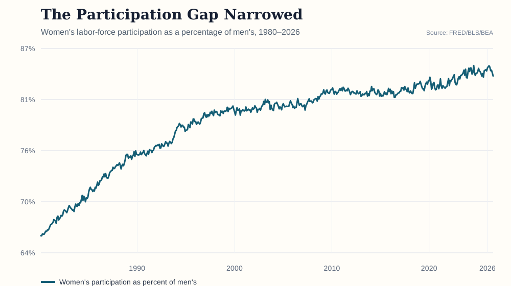
The first chart captures the extensive margin: who enters the labor market. In 1980, the participation rate for women age 20 and over was about 66% of the corresponding rate for men. By the end of the original study period it was approximately 82.5%; by August 2026 it was about 84.1%.
This convergence is not a complete measure of opportunity. Women and men differ in unpaid caregiving, health, age composition, family choices and other characteristics. Nor should equal participation be imposed as a mechanical target. The economic point is narrower: the enormous earlier gap could not plausibly have represented an equally enormous difference in useful talent. As legal, educational, occupational and social barriers weakened, millions of women entered market production. That directly increased the fraction of the population producing measured market output.
The more revealing question is whether entry occurred only into low-paid work. If it had, participation could increase while the economy continued to waste comparative advantage. The wage evidence says something more consequential happened.
2. Relative real earnings converged
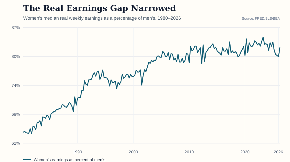
Among full-time wage and salary workers, women’s median real weekly earnings increased from about 63.4% of men’s in early 1980 to 81.9% at the end of 2010 and 82.4% in the latest quarter. Because this is a ratio of real wages, general inflation cannot explain the convergence.
Wages are not identical to productivity. Bargaining power, occupational rents, unions, minimum wages, monopsony, discrimination and selection into full-time employment all influence pay. Yet in the standard competitive model, the real wage is related to marginal product. When participation rises at the same time that relative real earnings rise, the evidence is inconsistent with a story in which women merely flooded into marginal, low-productivity work. It is consistent with occupational upgrading, increased education, improved matching and reduced discrimination—the very channels at the heart of the allocation model.
Composition is sometimes presented as a reason to dismiss the wage result: perhaps the women entering or remaining in full-time work became more educated or shifted into better occupations. But for this question, composition is not merely statistical noise. More education and movement into skilled occupations are part of the mechanism. The historical barriers described by Hsieh and his coauthors included barriers to acquiring occupation-specific human capital as well as discrimination in labor markets. If talented women become physicians, attorneys, scientists, professors and managers rather than being diverted elsewhere, both measured composition and productive capacity should change.
Still, this chart cannot tell us how much of the narrowing resulted from reduced discrimination, how much from education, how much from occupational choice, or how much from changes among men. A credible account must acknowledge that male participation declined over the period and that relative ratios can converge through movement in either numerator or denominator. That is why these charts corroborate the broad mechanism but do not replace microdata.
3. Productivity, living standards and wealth rose
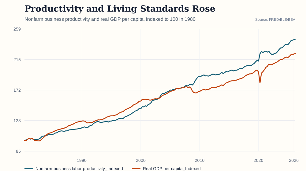
From 1980 through the end of 2010, nonfarm business labor productivity rose from 100 to approximately 193, while real GDP per person reached roughly 173. By the latest observations, those indexes were about 244 and 224. Real household wealth per person rose farther—from 100 in 1980 to about 218 in 2010 and 371 in the latest common observation.
It would be a mistake to draw a causal arrow directly from the first two charts to the third. Technology, capital, globalization, education, immigration, policy and financial markets all changed at the same time. Trending series can look persuasive even when their relationship is spurious. A regression in levels would flatter the thesis; a short-run regression in differences could throw away the slow structural change I am trying to understand.
Those are descriptive facts, not causal proof. Technology, capital, education, immigration, policy and financial markets were all changing. But the facts give us something concrete to test: participation widened, relative earnings improved, productivity and GDP rose, and real wealth compounded. The question is whether the timing inside a dynamic model follows the same route.
Putting the thesis into a VAR
RainbowStats should do more than draw rising lines. I put four variables into one vector autoregression: women’s participation relative to men’s, labor productivity, real GDP per person and real household wealth per person. I used quarterly log changes so common trends would not manufacture a result. A VAR treats every variable as endogenous:
| Feedback-loop path, 1980–present | VAR(2) sum | VAR(4) sum |
|---|---|---|
| Relative participation → labor productivity | +0.215 | +0.189 |
| Labor productivity → real wealth per person | +0.220 | +0.288 |
| Real wealth per person → real GDP per person | +0.174 | +0.191 |
| Real GDP per person → relative participation | +0.077 | +0.026 |
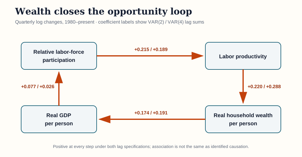
This is the result that changed the essay. Wealth does not merely sit at the end of the chain. Participation precedes productivity; productivity precedes wealth; wealth precedes GDP; and GDP precedes participation. All four links remain positive when I expand the window from two to four quarters.
The reverse link from GDP directly to wealth is negative over these short windows. That matters. The data do not support the lazy claim that every additional dollar of GDP immediately becomes household wealth. Asset prices, debt, housing and distribution intervene. The cleaner empirical route is productivity into wealth, and wealth back into economic activity and participation.
I will not call this causal proof. The model is small, omitted variables remain, and the current RainbowStats coefficient table does not report standard errors. What I can say is narrower: after differencing the data, admitting feedback and changing the lag length, the proposed loop keeps the predicted sign at every step. The thesis survives a serious first attempt to knock it down.
What the structural study actually found
| Hsieh–Hurst–Jones–Klenow result, 1960–2010 | Share of growth attributed to changing barriers |
|---|---|
| Market GDP per person, baseline specification | 41.5% |
| Market earnings per person | 38.4% |
| Market GDP per worker | 24.0% |
| Market plus home GDP per person | 32.7% |
| Market GDP per person, estimated preference heterogeneity | 37.4% |
| Market GDP per person, stronger preference heterogeneity | 28.3% |
The distinction between output per person and output per worker matters. Declining barriers raised participation, so the effect on market GDP per person is larger than the effect on productivity among those already working. In the baseline, changing barriers explain 41.5% of market GDP-per-person growth but 24% of market GDP-per-worker growth. This is exactly what the growth-accounting equation predicts: opportunity expands both the number of market participants and the productivity of their allocation.
The authors also find that white women account for most of the estimated contribution because they were a much larger share of the population than Black men or Black women. That is a demographic statement about the decomposition, not a judgment about the importance of civil rights. The study is limited to four groups—white men, white women, Black men and Black women—and therefore should not casually be summarized as covering all “people of color.” It does not separately analyze Hispanic, Asian, Indigenous or multiracial Americans.
The result depends on assumptions. The crucial identifying assumption is that relative innate occupational talent across groups remains stable over time. If women were dramatically less capable of becoming doctors in 1960 but their innate medical ability mysteriously converged toward men’s by 2010, the model would misclassify changing talent as declining barriers. The authors regard that story as implausible and test alternatives, including allowing gender differences in physically demanding occupations and allowing 2010 group differences to reflect talent rather than distortion. Their central growth result remains large under these alternatives.
That robustness does not transform the estimate into an experimental result. Structural models organize evidence through theory. Their value lies in making assumptions explicit and calculating counterfactuals that raw correlations cannot. The correct response is neither to treat 41.5% as revealed truth nor to dismiss it because it comes from a model. It is to ask whether the assumptions are reasonable, whether the observable implications fit the data, and whether alternative specifications leave the central conclusion intact.
Education, affirmative action and the meaning of merit
Durlauf also points to evidence from the University of California. Zachary Bleemer studied California’s Proposition 209, which ended race-based affirmative action at public universities. Using linked administrative records and a difference-in-differences design, he found that underrepresented minority applicants cascaded into lower-quality colleges, degree attainment declined, STEM completion declined and later wages fell. He also found no offsetting net benefit large enough among marginal white and Asian applicants to reverse the conclusion.
This evidence addresses an important objection: perhaps removing affirmative action simply reallocates scarce university seats toward more qualified students and therefore increases efficiency. Bleemer’s results suggest that this account is incomplete. Admission to a more productive educational environment can affect the human capital a student ultimately acquires. A rule that looks meritocratic when evaluated only at the admissions threshold can reduce total human-capital production if it places students where their development and completion outcomes are weaker.
I am not defending every program sold under the label “DEI.” The label covers practices of radically different quality; some may be bureaucratic, ineffective or counterproductive. Evidence that historical barriers were costly does not relieve any present program of a cost-benefit test. Merit remains the objective. The economic question is whether an institution finds and develops talent—or screens it out for reasons unrelated to productive ability.
But merit is an outcome of discovery as well as a property waiting to be observed. Test scores, prior schools, family wealth, networks, mentoring and information determine whose potential becomes visible. A genuinely meritocratic economy does not protect demographic representation for its own sake, nor does it pretend that the starting line has always been equal. It searches widely for comparative advantage, removes irrelevant barriers and evaluates programs by whether they expand capability and performance.
Why compounding closes the loop
Wealth is not merely the last line in an accounting exercise. It carries opportunity forward through time. A simple household wealth equation is:
Here (W) is wealth, (r) the return on existing assets, (s) the saving rate and (Y) income. Productive work raises income. Income permits saving and ownership. Returns compound what was saved. That wealth can finance education, housing, relocation, entrepreneurship and the ability to survive taking a risk. Compounding wealth therefore creates more opportunities—and begins the loop again.
But the word “ultimately” must do real work. GDP growth does not automatically become broadly distributed household wealth. Families with little disposable income may be unable to save. Asset ownership is unequal, so capital gains accrue disproportionately to those who already possess wealth. Housing access, credit conditions, medical costs, taxation and inheritance shape the conversion of income into net worth. Opportunity that raises wages is necessary for broad wealth creation, but it may not be sufficient.
That is why the distribution of wealth still matters. If added output accrues only to people who already own assets, the feedback into broad opportunity will be weak. Labor freed from arbitrary barriers can produce greater national wealth; converting that gain into widespread opportunity also requires access to saving, ownership and human-capital investment.
What current policy can and cannot be said to do
The Trump administration has explicitly ordered the termination of federal DEI programs and has framed its approach as restoring merit-based opportunity. Supporters argue that preferences can themselves become discriminatory, weaken standards and impose administrative costs. Those claims deserve empirical evaluation rather than dismissal. A policy branded as diversity-enhancing should not receive immunity from measurement.
Durlauf’s warning is about the opposite error: assuming that dismantling programs bearing the DEI label must increase merit and efficiency. The historical record shows that ostensibly neutral institutions can preserve severe misallocation. If current policy discourages qualified women or minority students and workers from education, research, public service or high-productivity occupations, the cost will not appear immediately in a monthly jobs report. Human-capital formation and occupational matching compound over years.
My charts cannot estimate the future effect of policies adopted in 2025 or 2026. The observations are too close to the policy changes, and broad national series cannot identify the affected groups or institutions. Anyone claiming that the charts already prove either large damage or no damage would be running ahead of the evidence.
What the history establishes is the size of the risk. The United States once left a remarkable quantity of ability underused. As barriers fell, participation and relative earnings converged while productivity and living standards rose. A structural model attributes a material portion of growth to that improved allocation. A separate quasi-experimental study finds that removing affirmative action from the University of California reduced educational attainment and later earnings for affected applicants without compensating gains for those allegedly crowded out. These findings do not dictate every policy detail, but they make complacency expensive.
What I think the evidence says
This began with Durlauf’s claim, but I did not want to publish a paraphrase of somebody else’s model. The public data establish five facts. Women’s participation relative to men’s rose from approximately 66% to 84%. Women’s real weekly earnings rose from about 63% to 82% of men’s. Labor productivity more than doubled. Real GDP per person more than doubled. Real household wealth per person more than tripled.
The VAR adds something the charts cannot. It finds a complete positive loop: participation leads productivity, productivity leads wealth, wealth leads GDP, and GDP leads participation. The loop survives when I extend the lag window from two quarters to four. Wealth is not simply the destination. Compounded wealth helps finance the next round of participation and productive work.
I will not call that proof in the mathematical sense. The model does not isolate a policy shock, and the displayed coefficients still need formal uncertainty estimates. But it does more than place rising lines beside one another. It differences the data, admits feedback and asks whether the sequence appears in time. The predicted loop remains visible under both lag specifications.
This is a Chicago argument in the best sense. Barriers distort choices. Misallocated ability is wasted capital. Diversity has economic value when it reveals and deploys talent that arbitrary barriers concealed. That is not a retreat from meritocracy; it is how a serious meritocracy searches for comparative advantage.
Durlauf is right to put opportunity inside the growth debate. The cost of exclusion is not confined to the person excluded. It appears as a job poorly matched, an education never completed, an invention never pursued, a business never formed and a smaller base from which wealth can compound. The loss then reaches the next generation, which begins with fewer choices.
That gives me a measurable standard. Are talented people reaching the education and occupations where they contribute most? Does wider participation precede productivity? Does productivity become wealth? Does accumulated wealth create new opportunity? A program bearing the label “DEI” should not be presumed effective—but a policy that closes opportunity should not be presumed costless.
Replication script
The full script below generates the three historical charts and the two- and four-lag wealth-loop models, automatically extending the series through the latest observations. The earlier saved analysis remains available; the revised program is reproduced in full here.
MenParticipation=SET_NAME(LNS11300001,"Men age 20+")
WomenParticipation=SET_NAME(LNS11300002,"Women age 20+")
ParticipationData=SAME_DATE_RANGE(LIST(MenParticipation,WomenParticipation))
MenParticipation=EX(ParticipationData,series:0)
WomenParticipation=EX(ParticipationData,series:1)
ParticipationRatio=SET_NAME(100*WomenParticipation/MenParticipation,"Women's participation as percent of men's")
ParticipationRatio=SERIES_SINCE(ParticipationRatio,19800101)
ParticipationChart=LINE_CHART(ParticipationRatio)
ParticipationChart=SET_TITLE_SUBTITLE(ParticipationChart,"The Labor-Force Participation Gap Narrowed","Women's participation as a percentage of men's; monthly, 1980 to latest observation")
ParticipationChart=PUBLICATION_CHART(ParticipationChart)

MenWage=SET_NAME(LES1252881900Q,"Men")
WomenWage=SET_NAME(LES1252882800Q,"Women")
WageData=SAME_DATE_RANGE(LIST(MenWage,WomenWage))
MenWage=EX(WageData,series:0)
WomenWage=EX(WageData,series:1)
WageRatio=SET_NAME(100*WomenWage/MenWage,"Women's earnings as percent of men's")
WageRatio=SERIES_SINCE(WageRatio,19800101)
WageChart=LINE_CHART(WageRatio)
WageChart=SET_TITLE_SUBTITLE(WageChart,"The Real Earnings Gap Narrowed","Median weekly real earnings of full-time workers; quarterly, 1980 to latest observation")
WageChart=PUBLICATION_CHART(WageChart)

Productivity=SET_NAME(OPHNFB,"Nonfarm business labor productivity")
RealGDPPerCapita=SET_NAME(A939RX0Q048SBEA,"Real GDP per capita")
Population=TO_QUARTERLY(POP)
PriceLevel=GDPDEF
RealWealthPerCapita=SET_NAME(100*TNWBSHNO/Population/PriceLevel,"Real household wealth per capita")
GrowthData=SAME_DATE_RANGE(LIST(Productivity,RealGDPPerCapita,RealWealthPerCapita))
GrowthData=SERIES_SINCE(GrowthData,19800101)
GrowthData=INDEX_100(GrowthData)
GrowthChart=LINE_CHART(GrowthData)
GrowthChart=SET_TITLE_SUBTITLE(GrowthChart,"Productivity, GDP and Wealth Rose","All series indexed to 100 in 1980; quarterly through latest common observation")
GrowthChart=PUBLICATION_CHART(GrowthChart)

ParticipationRatioQuarterly=TO_QUARTERLY(ParticipationRatio)
WealthLoopData=SAME_DATE_RANGE(LIST(ParticipationRatioQuarterly,Productivity,RealGDPPerCapita,RealWealthPerCapita))
WealthLoopGrowth=LOGDIFF(WealthLoopData)
WealthLoopVAR2=VAR_MODEL(WealthLoopGrowth,2)
WealthLoopVAR4=VAR_MODEL(WealthLoopGrowth,4)

SLIDESHOW(ParticipationChart,WageChart,GrowthChart,WealthLoopVAR2,WealthLoopVAR4)
Sources and limitations
- Adam Smith, The Wealth of Nations, Introduction and Plan, and Book I, Chapter V, 1776.
- Steven N. Durlauf, “Three Ways Trump Is Strangling Economic Growth,” The New York Times, July 2, 2026.
- Chang-Tai Hsieh, Erik Hurst, Charles I. Jones and Peter J. Klenow, “The Allocation of Talent and U.S. Economic Growth,” Econometrica 87(5), 2019.
- Zachary Bleemer, “Affirmative Action, Mismatch, and Economic Mobility after California’s Proposition 209,” Quarterly Journal of Economics 137(1), 2022.
- University of Chicago Harris School of Public Policy, Steven Durlauf faculty profile.
- FRED/BLS: men’s and women’s labor-force participation; men’s and women’s median real weekly earnings; nonfarm business labor productivity.
- FRED/BEA: real GDP per capita.
- Federal Reserve Financial Accounts and FRED: household and nonprofit net worth, population and the GDP deflator.
Limitations: The charts and VAR use broad aggregate series. They do not adjust for occupation, education, age composition, hours, selection, household structure or the distribution of wealth. Household net worth includes asset-price changes as well as saving. The VAR coefficients describe conditional dynamics, not identified policy effects; the current coefficient table does not supply standard errors. The structural and quasi-experimental papers provide stronger identification, but their conclusions also remain conditional on their data, assumptions and institutional settings.