The epicycles command reconstructs a time series using a selected set of dominant spectral cycles.
Inspired by the classical Fourier epicycle visualization, the command decomposes a series into periodic components and then animates how those cycles combine to recreate the observed data.
The visualization is both an educational tool and a diagnostic tool. It helps reveal how much of a series can be explained by recurring cyclical behavior and how many spectral components are required to approximate the original observations.
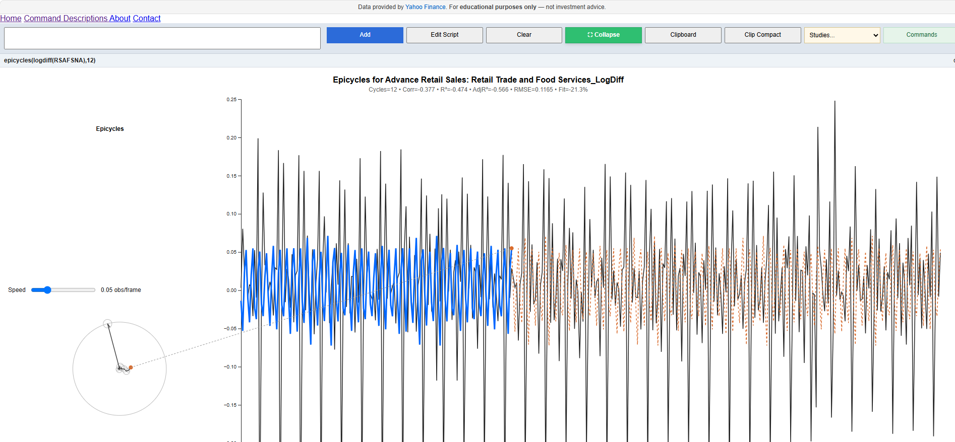
epicycles(logdiff(RSAFSNA),12)This example analyzes the monthly growth rate of U.S. Advance Retail Sales (not seasonally adjusted). The animation reconstructs the series using the twelve strongest spectral cycles identified in the frequency domain.
epicycles(series, numCycles)Where:
The command produces an animated panel consisting of:
The circular diagram on the left shows a chain of rotating vectors. Each vector represents a dominant cycle extracted from the spectrum of the series.
The endpoint of the final vector traces the reconstructed value generated by the combined cycles. A dashed guide line links the epicycle endpoint to the corresponding fitted value on the time series chart.
The chart on the right compares:
As the animation progresses, users can visually observe how cyclical components combine to recreate the original signal.
Several goodness-of-fit measures are displayed beneath the title:
Increasing the number of cycles generally improves the reconstruction, but at the cost of greater complexity. Adjusted R² helps determine whether additional cycles are contributing meaningful explanatory power.
Many economic and financial time series contain recurring periodic behavior. The epicycle reconstruction provides a visual measure of how much of the observed variation can be attributed to cyclical structure versus irregular noise.
Series with strong business-cycle, seasonal, or market-cycle effects often achieve good fits with relatively few cycles. Highly noisy series may require dozens of cycles and still exhibit modest explanatory power.
The command can therefore be viewed as a form of spectral compression analysis:
The command is based on the spectral decomposition of the input series. The reconstruction is not intended as a forecasting model; rather, it illustrates how much of the historical variation can be explained by recurring frequencies.
For highly seasonal series, dominant annual and semi-annual cycles may account for a substantial portion of the reconstruction. For financial returns and other noisy processes, significantly more cycles may be required to achieve meaningful explanatory power.