The regression command estimates a linear relationship between time series. It compares an observed dependent series with one or more explanatory series, then reports fitted values, residuals, regression coefficients, standard errors, t-statistics, and model diagnostics.
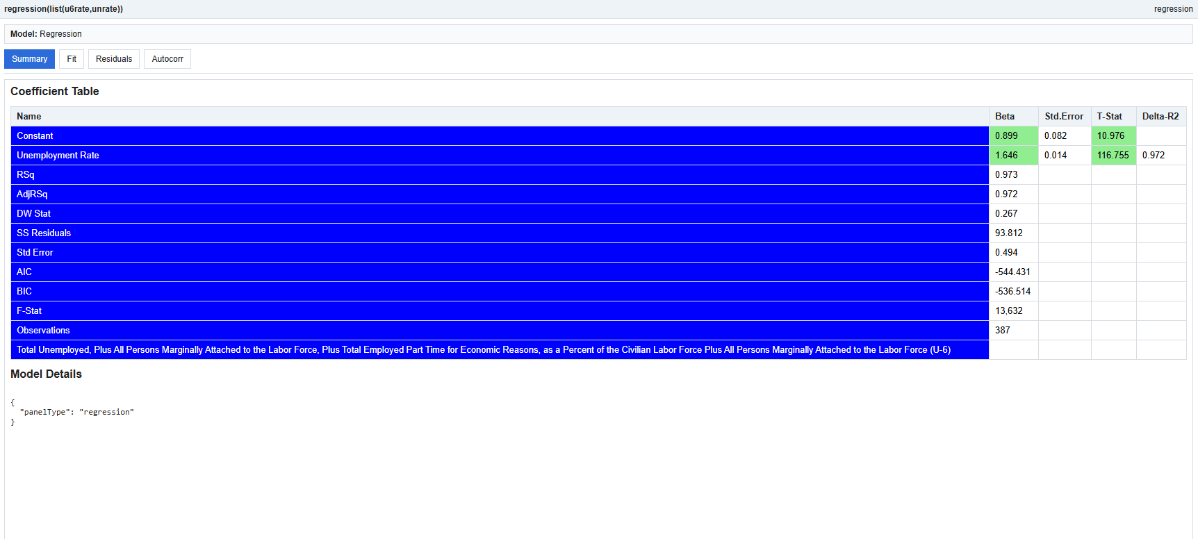
regression(LIST(UNRATE,U6RATE))This example estimates a regression relationship between the unemployment rate and the U-6 unemployment measure.
regression(seriesList)The input should be a list of time series. The first series is treated as the dependent variable. The remaining series are used as explanatory variables. A constant term is added automatically.
The command produces a regression panel including:
The fitted chart compares the observed series with the model’s predicted values. A close fit means the regression explains much of the movement in the dependent series.
The residual chart shows what the model did not explain. Residuals should ideally look centered around zero without an obvious pattern.
The autocorrelation chart helps identify whether residuals remain serially correlated. Large residual autocorrelations may indicate that the model is missing time-series structure.
Regression is useful for estimating linear relationships, measuring factor exposure, and testing whether one series helps explain another. Coefficients show the estimated sensitivity of the dependent variable to each explanatory variable.
A statistically significant coefficient suggests that the explanatory series has useful information in the sample. However, statistical significance does not by itself prove causation.
The regression command is exploratory and diagnostic. Results should be interpreted with attention to sample size, data frequency, stationarity, omitted variables, and economic reasoning.