Replicating selected parts of research papers has become one of my most useful ways to develop RainbowStats. A real economic question exercises the entire system: data retrieval, transformations, estimation, diagnostics and presentation. We find bugs, add models and make the commands clearer for the MCP assistant. This exercise began with a 110-page paper on oil prices—and ended with better tools for studying them.
Romain Houssa and Jolan Mohimont’s Oil Prices and Global Activity in a General Equilibrium Model with Dynamic Elasticities (15 October 2026) asks how gradually changing supply and demand responses affect oil prices and activity. Wells take time to develop; consumers take time to replace equipment. The authors incorporate those adjustments into a general-equilibrium model and estimate it with Bayesian methods.
Their central finding is that assumptions and information about elasticities beyond the impact month matter for the importance assigned to different shocks. Informative elasticity priors, or drilling information under diffuse priors, support supply responsiveness that rises with the horizon. That is a useful idea to explore with a smaller, transparent exercise.
Start with the data
Using the paper’s January 1975–December 2019 window, I assembled US crude production, industrial production, real crude prices and inventories from EIA and FRED. These are accessible US substitutes for the paper’s global dataset. They provide 540 monthly observations before lag losses.
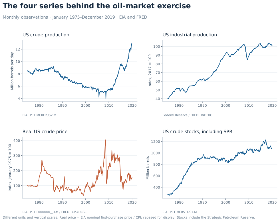
The decline and later recovery of US production, large oil-price swings and long accumulation of crude inventories are visible before any model is fitted. Total stocks include the Strategic Petroleum Reserve, so this series combines commercial storage and public stockpiling. The appendix lists the source codes and transformations.
The new VECM_MODEL diagnostics let us examine long-run combinations and short-run adjustment together. Here, a levels VAR order of 13 means 12 lagged differences, with one assumed cointegrating relation and 527 fitted observations. The chart compares observed monthly log changes with the model’s fitted changes.
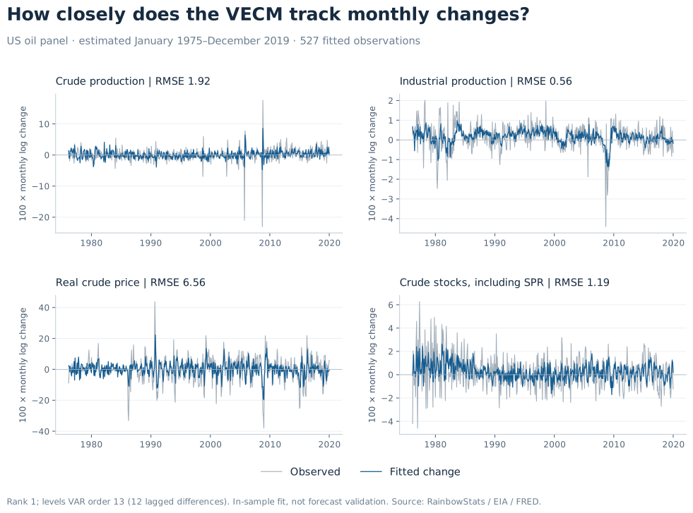
The diagnostics add necessary context. At the 5% level, both Johansen tests select rank two at order 12 and rank one at order 13. The order-13 model has stable transient dynamics, but its residual-whiteness test returns p = 0.000832. Our simple US specification still needs work on seasonality, inventory behavior and structural change. These results assess our substitute model; they do not evaluate the authors’ estimated model.
Then ask what caused the price rise
The DSGE operator lets us move from fitted associations to explicit economic scenarios. I built a calibrated oil-market subsystem in which production, consumption, storage and a simplified activity measure determine prices jointly. Its equations incorporate forward-looking storage and investment. It is an educational extension, not a reproduction of the paper’s full household-and-capital model or Bayesian estimates.
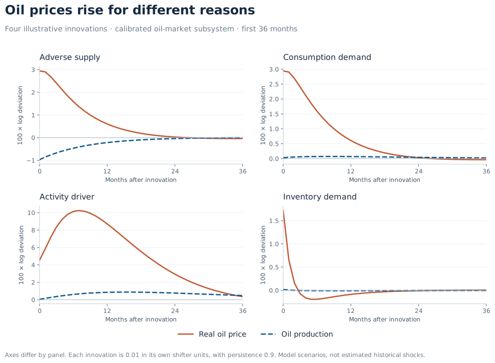
An adverse supply innovation initially reduces production by about 0.97% and raises the real price by about 2.94%. A consumption-demand innovation raises prices while production edges up. An activity-driver innovation raises both activity and oil demand; an inventory-demand innovation initially raises prices as oil moves into storage. These percentages approximate log deviations from the model’s steady state.
In this simplified system, equal-sized supply and consumption-demand shifters produce identical price paths, despite different quantity responses. Prices alone therefore cannot distinguish those two scenarios here. The labels come from the imposed equations, not an identification of historical events.
The adjustment horizon matters
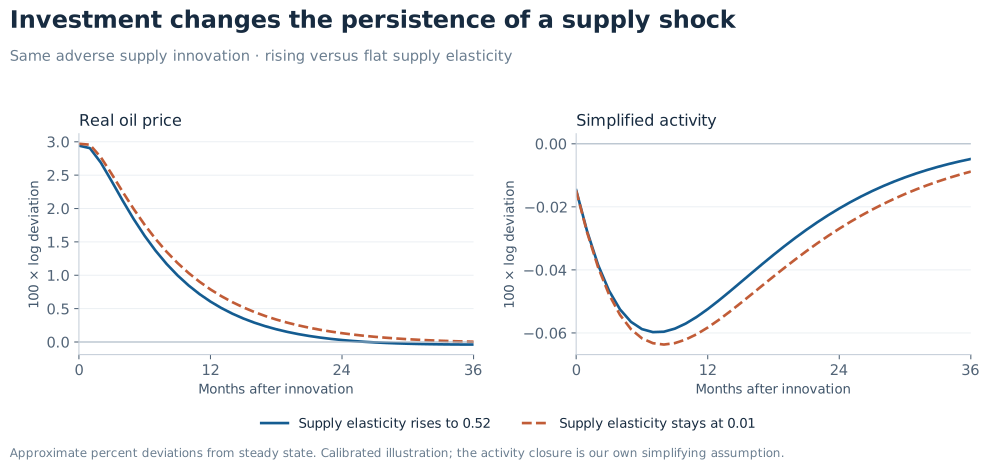
Allowing supply elasticity to rise from 0.01 toward 0.52 changes the persistence of the adverse supply response. At month 12, the price increase is about 0.61%, compared with 0.79% when supply elasticity stays at 0.01. The chart also shows the associated response of our simplified activity measure.
The paper supplied the economic question. Working through it improved the VECM diagnostics, sharpened the DSGE examples, clarified lag conventions for the MCP and even exposed a table-rendering bug. That is a development benefit of replication: the research teaches us something about the economy while helping us build tools that explain it more clearly.
Try the exercise. Open the saved RainbowStats study to explore it directly, or download the script and paste it into the script editor. The final command builds a slideshow with model diagnostics, fitted changes and five shock charts.
Full RainbowStats script · 70 equations
PriceRaw=EIA(PET.F000000__3.M)
OutputRaw=EIA(PET.MCRFPUS2.M)
StocksRaw=EIA(PET.MCRSTUS1.M)
Raw=SAME_DATE_RANGE(OutputRaw,INDPRO,PriceRaw,StocksRaw,CPIAUCSL)
Output=SET_NAME(GET_SERIES(Raw,0),"US crude production")
Activity=SET_NAME(GET_SERIES(Raw,1),"US industrial production")
RealPrice=SET_NAME(GET_SERIES(Raw,2)/GET_SERIES(Raw,4),"Real US crude price")
Stocks=SET_NAME(GET_SERIES(Raw,3),"US crude stocks including SPR")
USLevels=SERIES_BETWEEN(SAME_DATE_RANGE(LOG(Output),LOG(Activity),LOG(RealPrice),LOG(Stocks)),19750101,20191231)
EC=VECM_MODEL(USLevels,13,1)
EC12=VECM_MODEL(USLevels,12,1)
FitSlides=EXTRACT(EC,"slideshow")
Rank13=EXTRACT(EC,"rank_test")
Rank12=EXTRACT(EC12,"rank_test")
UnitRoots=EXTRACT(EC,"unit_root")
LagSearch=EXTRACT(EC,"lag_selection:24")
ResidualCheck=EXTRACT(EC,"autocorrelation:36")
RootCheck=EXTRACT(EC,"stability")
EQ=DSGE_MODEL()
EQ=ADD_DSGE_SHOCK(EQ,"EPS_SUPPLY")
EQ=ADD_DSGE_SHOCK(EQ,"EPS_ACTIVITY")
EQ=ADD_DSGE_SHOCK(EQ,"EPS_DEMAND")
EQ=ADD_DSGE_SHOCK(EQ,"EPS_INVENTORY")
EQ=ADD_DSGE_EQUATION(EQ,"KS=0.962*LAG(KS,1)+0.01938*LAG(RS,1)")
EQ=ADD_DSGE_EQUATION(EQ,"KD=0.967*LAG(KD,1)+0.00627*LAG(RD,1)")
EQ=ADD_DSGE_EQUATION(EQ,"Q=0.01*P+KS+ZS")
EQ=ADD_DSGE_EQUATION(EQ,"C=Y-0.26*P-KD+ZD")
EQ=ADD_DSGE_EQUATION(EQ,"V=0.46*(0.87*LEAD(P,1)-P)+ZV")
EQ=ADD_DSGE_EQUATION(EQ,"V-LAG(V,1)=Q-C")
EQ=ADD_DSGE_EQUATION(EQ,"Y=0.9*LAG(Y,1)-0.005*P+ZA")
EQ=ADD_DSGE_EQUATION(EQ,"ZS=0.9*LAG(ZS,1)-0.01*EPS_SUPPLY")
EQ=ADD_DSGE_EQUATION(EQ,"ZA=0.9*LAG(ZA,1)+0.01*EPS_ACTIVITY")
EQ=ADD_DSGE_EQUATION(EQ,"ZD=0.9*LAG(ZD,1)+0.01*EPS_DEMAND")
EQ=ADD_DSGE_EQUATION(EQ,"ZV=0.9*LAG(ZV,1)+0.01*EPS_INVENTORY")
EQ=ADD_DSGE_EQUATION(EQ,"RS=0.04121741533708234*LEAD(P,1)+0.9587825846629177*LEAD(RS,1)")
EQ=ADD_DSGE_EQUATION(EQ,"RD=0.03623413787001928*LEAD(P,1)+0.9637658621299807*LEAD(RD,1)")
EQ=COMPILE_DSGE(EQ)
EQ=CONFIGURE(EQ,"IMPULSE_HORIZON",120)
EQ=SOLVE_DSGE(EQ)
EQFlat=DSGE_MODEL()
EQFlat=ADD_DSGE_SHOCK(EQFlat,"EPS_SUPPLY")
EQFlat=ADD_DSGE_SHOCK(EQFlat,"EPS_ACTIVITY")
EQFlat=ADD_DSGE_SHOCK(EQFlat,"EPS_DEMAND")
EQFlat=ADD_DSGE_SHOCK(EQFlat,"EPS_INVENTORY")
EQFlat=ADD_DSGE_EQUATION(EQFlat,"KS=0.962*LAG(KS,1)+0*LAG(RS,1)")
EQFlat=ADD_DSGE_EQUATION(EQFlat,"KD=0.967*LAG(KD,1)+0.00627*LAG(RD,1)")
EQFlat=ADD_DSGE_EQUATION(EQFlat,"Q=0.01*P+KS+ZS")
EQFlat=ADD_DSGE_EQUATION(EQFlat,"C=Y-0.26*P-KD+ZD")
EQFlat=ADD_DSGE_EQUATION(EQFlat,"V=0.46*(0.87*LEAD(P,1)-P)+ZV")
EQFlat=ADD_DSGE_EQUATION(EQFlat,"V-LAG(V,1)=Q-C")
EQFlat=ADD_DSGE_EQUATION(EQFlat,"Y=0.9*LAG(Y,1)-0.005*P+ZA")
EQFlat=ADD_DSGE_EQUATION(EQFlat,"ZS=0.9*LAG(ZS,1)-0.01*EPS_SUPPLY")
EQFlat=ADD_DSGE_EQUATION(EQFlat,"ZA=0.9*LAG(ZA,1)+0.01*EPS_ACTIVITY")
EQFlat=ADD_DSGE_EQUATION(EQFlat,"ZD=0.9*LAG(ZD,1)+0.01*EPS_DEMAND")
EQFlat=ADD_DSGE_EQUATION(EQFlat,"ZV=0.9*LAG(ZV,1)+0.01*EPS_INVENTORY")
EQFlat=ADD_DSGE_EQUATION(EQFlat,"RS=0.04121741533708234*LEAD(P,1)+0.9587825846629177*LEAD(RS,1)")
EQFlat=ADD_DSGE_EQUATION(EQFlat,"RD=0.03623413787001928*LEAD(P,1)+0.9637658621299807*LEAD(RD,1)")
EQFlat=COMPILE_DSGE(EQFlat)
EQFlat=CONFIGURE(EQFlat,"IMPULSE_HORIZON",120)
EQFlat=SOLVE_DSGE(EQFlat)
Opening=TEXT_SLIDE("Replication improves the tools","A selective exercise inspired by Houssa and Mohimont, Oil Prices and Global Activity in a General Equilibrium Model with Dynamic Elasticities, 15 October 2026.","The data models below use US substitutes over January 1975 to December 2019. The calibrated oil-market subsystem is an educational scenario model; it does not reproduce the authors' full RBC model, Bayesian estimation or historical shock decomposition.")
Methods=TEXT_SLIDE("VECM: levels, changes and diagnostics","EC uses four log-level variables and rank one. Its levels VAR order 13 includes 12 lagged differences. EC12 uses 11 lagged differences; compare the rank tests.","Fitted values are in-sample monthly log changes, not fitted price levels or out-of-sample forecasts. The data use current revisions. EIA oil series are not seasonally adjusted; INDPRO and CPI are.","Native tests select rank one at order 13 and rank two at order 12. At order 13 residual whiteness is rejected (p about 0.000832), despite stable transient roots. Inventory integration, seasonality and structural change need further study.")
ScenarioNotes=TEXT_SLIDE("How to read the shocks","P is real oil price, Q production, C consumption, V inventories and Y a simplified activity measure. Responses are log deviations; 0.01 is approximately one percent. Month zero is the impact month.","Supply, consumption-demand, activity and inventory shifters each have persistence 0.9. Shock magnitudes are 0.01 in their own shifter units. They are not equally sized observed GDP or production changes.","Supply elasticity rises from 0.01 to 0.52; demand moves from -0.26 to -0.45. The flat-supply comparison keeps supply elasticity at 0.01. The activity equation is our simplifying closure, not the paper's household-and-capital block.","Equal-sized supply and consumption-demand shifters have the same price path in this simplified model. The solver checks a stable solution but does not test Blanchard-Kahn determinacy. These are illustrative mechanisms, not identified historical shocks.")
Solver=EXTRACT(EQ,"solver_summary")
SupplyShock=SET_TITLE(EXTRACT(EQ,"impulse_response_chart_EPS_SUPPLY"),"Illustrative adverse supply shock")
DemandShock=SET_TITLE(EXTRACT(EQ,"impulse_response_chart_EPS_DEMAND"),"Illustrative consumption-demand shock")
ActivityShock=SET_TITLE(EXTRACT(EQ,"impulse_response_chart_EPS_ACTIVITY"),"Illustrative activity-driver shock")
InventoryShock=SET_TITLE(EXTRACT(EQ,"impulse_response_chart_EPS_INVENTORY"),"Illustrative inventory-demand shock")
FlatSupplyShock=SET_TITLE(EXTRACT(EQFlat,"impulse_response_chart_EPS_SUPPLY"),"Adverse supply shock with flat supply elasticity")
SLIDE(Opening,Methods,Rank12,Rank13,UnitRoots,LagSearch,ResidualCheck,RootCheck,FitSlides,ScenarioNotes,Solver,SupplyShock,DemandShock,ActivityShock,InventoryShock,FlatSupplyShock)
For readers who want to go further
Appendix: what the findings tell us
A. The paper’s contribution and this exercise
The authors study a global oil market in general equilibrium, with economic decisions governing drilling, oil-saving capital and storage. Their Bayesian exercise examines how elasticity priors and the information set change the shocks to which oil-price and activity fluctuations are attributed. A small impact supply elasticity need not imply that producers remain equally unresponsive a year later. Drilling information helps discipline that distinction.
Our exercise takes that horizon-dependent adjustment mechanism as its starting point. The VECM uses US substitutes to explore the data, and the DSGE operator solves a smaller calibrated system. We have not reproduced the authors’ posterior distributions, historical shock decomposition or forecast-error variance shares. Those would require their complete data construction, model and estimation procedure. The new graphs illustrate the mechanism under stated assumptions.
B. Data: what is actually in each chart?
All four inputs are monthly and use January 1975–December 2019. Figure 1 displays their levels; the VECM takes logarithms internally supplied by the script. First differences of those logs are the fitted quantities in Figure 2. The baseline uses US data throughout.
| Input | Source and identifier | Display and model treatment |
|---|---|---|
| Crude production | EIA PET.MCRFPUS2.M | Original thousand barrels/day; Figure 1 shows million barrels/day. Model input: log production. |
| Industrial production | Federal Reserve via FRED INDPRO | Seasonally adjusted index, 2017 = 100. Model input: log index. |
| Real crude price | EIA PET.F000000__3.M; BLS via FRED CPIAUCSL | US nominal first-purchase price divided by CPI. Figure 1 rebases that ratio to January 1975 = 100; the VECM uses its log without this display rebasing. |
| Crude inventories | EIA PET.MCRSTUS1.M | Total crude stocks including SPR, originally thousand barrels; Figure 1 shows million barrels. Model input: log stocks. |
Oil data are retrieved through EIA Open Data. EIA oil series are not seasonally adjusted here; INDPRO and CPI are. The domestic first-purchase price is a US measure, not a global oil benchmark. SPR accumulation, shale production and other regime changes can influence full-sample relationships. Inventories enter our VECM as log levels; the paper also uses inventory changes scaled by lagged production. These construction differences matter when interpreting coefficients.
C. Rank, adjustment and the quality of fit
The supplied rank is an explicit modeling choice. Native Johansen diagnostics give the following sensitivity result, using an unrestricted intercept in the change equations and no deterministic trend:
| Levels VAR order | Lagged differences | Trace rank at 5% | Max-eigen rank at 5% |
|---|---|---|---|
| 12 | 11 | 2 | 2 |
| 13 | 12 | 1 | 1 |
At order 13 and rank one, 540 observations leave 527 fitted changes. The largest transient companion-root modulus is about 0.98925, with the expected three unit roots. The adjusted portmanteau test at 36 residual lags nevertheless rejects whiteness (p = 0.000832). Stable propagation and residual whiteness answer different questions. An attractive fit cannot replace those checks.
Inventory integration deserves particular care: in our archived ADF checks, the level-test conclusion changes when a trend is included. A stationary component can contribute to the estimated rank. A normalized cointegrating vector therefore should not automatically be labeled an oil-demand or oil-supply elasticity. The useful next investigations are seasonal specification, inventory definitions and stability across economic regimes.
D. What the four innovations do on impact
Entries below are 100 times log deviations from steady state, approximately percent changes. Each innovation is 0.01 in its own shifter units, and its shifter decays with persistence 0.9. The normalization does not make the innovations equal observed production or GDP shocks.
| Innovation | Price | Production | Inventories | Simplified activity |
|---|---|---|---|---|
| Adverse supply | +2.942 | -0.971 | -0.191 | -0.015 |
| Consumption demand | +2.942 | +0.029 | -0.191 | -0.015 |
| Activity driver | +4.533 | +0.045 | +0.247 | +0.977 |
| Inventory demand | +1.717 | +0.017 | +0.472 | -0.009 |
The adverse supply shifter removes oil; inventories and consumption fall as the price rises. A consumption-demand shifter instead increases consumption, drawing on inventories while higher prices encourage production. Inventory demand initially shifts oil into storage. The activity driver raises our simplified activity measure and its demand for oil. The activity equation is an illustrative closure, so its response is not an estimated GDP effect from the paper.
Equal-sized supply and consumption-demand shifters generate the same price path in this subsystem. Their quantity responses differ. That feature limits what this simplified structure can identify; it also illustrates why production, stocks and activity belong beside prices in an oil-market discussion. The response lines have no estimated uncertainty bands.
E. Why changing the horizon changes the answer
The supply-capacity recurrence is calibrated so that a permanent price change raises supply elasticity from 0.01 toward 0.52, with monthly well decay 0.038. The signed demand elasticity moves from −0.26 toward −0.45 as oil-saving capital adjusts. Those permanent-price elasticity paths are distinct from the temporary equilibrium innovations in Figures 3 and 4.
In the adverse supply scenario, rising supply responsiveness reduces the remaining price effect at month 12 to about 0.605%, versus 0.787% under flat supply elasticity. At month 24 the effects are approximately 0.029% and 0.132%. The comparison holds the other subsystem assumptions fixed; it illustrates a channel, rather than estimating its historical contribution.
F. What the numerical checks establish
The native VECM fitted changes match an independent statsmodels calculation to numerical precision. Exported responses satisfy the subsystem’s 13 equations, including market clearing and the forward-looking storage and investment conditions, with discrepancies below 10−12. The selected DSGE transition is stable, with spectral radius about 0.96594. The solver does not test Blanchard–Kahn determinacy, so a stable computed transition alone does not establish a unique rational-expectations equilibrium.
These implementation checks and the statistical diagnostics serve different purposes. Together they make the exercise easier to reproduce and the assumptions easier to inspect. That is the practical development benefit of returning to research papers.
Source and methods
Paper: Houssa, Romain, and Jolan Mohimont. Oil Prices and Global Activity in a General Equilibrium Model with Dynamic Elasticities. Version dated 15 October 2026. See Figure 3; equations (7), (15) and (18); Tables 3 and 6; and Appendices B.4 and B.7. The supplied PDF contains a title page plus 110 numbered pages. The paper is not redistributed in this package.
Data: EIA monthly codes PET.MCRFPUS2.M (US crude production), PET.F000000__3.M (US crude first-purchase price) and PET.MCRSTUS1.M (total US crude stocks including SPR); FRED INDPRO and CPIAUCSL. Real price is nominal price divided by CPI. EIA oil series are not seasonally adjusted here. The data are current-vintage revisions, not historical real-time vintages.
Calibration: Supply elasticities 0.01 and 0.52; signed demand elasticities −0.26 and −0.45; monthly well decay 0.038; oil-saving capital depreciation 0.033; monthly discount factor 0.991/3; storage parameters 0.46 and 0.13; normalized inventory/production ratio one. Some elasticity values illustrate the paper’s prior centers, not posterior estimates. The activity equation Y=0.9*LAG(Y,1)-0.005*P+ZA and shock persistence 0.9 are our illustrative assumptions. The flat-supply variant removes the investment response of supply capacity.
Verification: All 70 script equations executed successfully through production RainbowStats on 30 October 2026. The native VECM fitted changes agree with an independent statsmodels calculation within 2 × 10⁻¹⁵ in log-change units. The archived shock paths satisfy the 13 subsystem equations with maximum discrepancies below 10−12. The solved transition is stable; the solver does not test Blanchard–Kahn determinacy. Neither numerical agreement nor stability establishes structural identification or a unique equilibrium.