In June, I thought it might be a fun exercise to build a market-making simulator. I had spent years trading derivatives. Could I put some of that experience into a game—one that lets someone feel the difference between getting a good trade and managing a good book?
The project grew. First came orders, partial fills, positions and cash balances. Then options, complex strategies, delta hedges, clearing controls and a pit full of competing traders. It now has a name: So, you want to be a market-maker.
The premise is simple. A broker brings business into the pit. You receive a share of it, along with an initial pricing edge. Your task is to manage the resulting inventory as the market changes. You can hedge, trade options against options, or carry some exposure. Every adjustment has a price.
Getting the edge is the beginning of the trade. Keeping it is the job.
The broker keeps you in business
A market-maker cannot wait indefinitely for a favorite bet. The broker returns with another order, and the new position may upset a book that looked comfortable a moment ago.
The simulator’s broker generates orders at random times, targeting roughly two allocations per simulated hour on average. These include individual calls and puts, straddles, strangles, vertical spreads and ratio structures. Broker business is distributed among the human participants and automated traders. Clearing capacity can limit an allocation, with the remainder offered to other traders.
That is close to the problem I wanted to recreate from the pit: a broker steps in with a large order and divides it among the crowd. You may like the trade, but you still have to fit it into everything you already own.
Suppose you receive a sale of an at-the-money straddle. You have collected premium and perhaps some edge. You have also taken on short gamma and short vega. An underlying hedge can reduce the initial delta. It cannot remove those other exposures.
Old market events at a current spot level
The replay applies historical percentage movements to a current starting index level. A crisis does not have to begin at the index price printed in an old newspaper. Its sequence of daily returns can be experienced at today’s price scale, with a new set of option strikes and expirations.
For each replay day, the engine takes the historical log return and sets a target closing level. It generates intraday fluctuations, scaled using the scenario’s volatility estimate, whose cumulative contribution is zero. The path can move around during the session while preserving that day’s historical close-to-close return.
For example, a historical decline of 10% turns a simulated opening level of 8,000 into a closing target of 7,200. What matters for the exercise is the relative move and the risk it creates in your current book.
The available scenarios include crashes, recoveries and sharp rallies. A short-gamma book can be uncomfortable on the way up as well as on the way down.
What is historical, and what is simulated? The daily return sequence comes from history. The intraday path, broker flow, option quotes and trading activity are generated. This is a historical scenario exercise, rather than a reconstruction of every transaction or option quote from the original event.
A variance-gamma option market
The option-pricing engine uses a variance-gamma model. Compared with a simple lognormal return model, it provides additional control over asymmetry and tail behavior. That makes it useful for constructing an option market with a volatility smile or skew. The model was developed by Dilip Madan, Peter Carr and Eric Chang.1
The engine uses the fast Fourier transform to calculate a grid of option values across strikes, following the approach associated with Carr and Madan.2 Those model values support the simulated option market as spot, time to expiry and the pricing assumptions change.
There are two distinct ingredients here. The historical replay supplies the market scenario. The pricing model supplies values for the options in that scenario. Using variance-gamma option prices does not mean that the generated intraday replay is itself an unconstrained variance-gamma price path.
That distinction matters when interpreting the results. The simulator is a place to explore how a strategy behaves under stated assumptions. Its prices are model prices, and its losses and profits belong to that simulated market.
The clearing firm has a vote
Market-makers can carry substantial leverage. A nearly delta-neutral book may still contain enormous exposure to a large move. My clearing firm wanted to know what happened to the book if the market fell 20%—and whether we had the capital to cover the loss.
The simulator puts that question into its clearing risk manager. It reprices the portfolio at a spot level 20% below the current market, holding time to expiry and each strike’s implied volatility unchanged for this test. It includes cash, option positions and the underlying, with the appropriate contract multipliers.
A compliant book must retain nonnegative equity under that stress. Active option books also have a deliberately simple inventory requirement: net put count must be positive. Long puts count positively; short puts count negatively, including legs inside complex strategies.
This reflects another rule from my trading experience: do not run a negative put count. The rule does not require one particular strike. Far out-of-the-money puts can be handy, but the trader can choose the contracts, provided the complete book satisfies the constraints.
Put count alone is not a measure of crash protection. Strikes, expirations and sizes matter. That is why the count rule sits alongside a full stress revaluation. The single down-20% scenario is also a simplified game constraint, not a complete description of real-world clearing margin or every possible market shock.
Checking the package matters. An option trade and its hedge belong together economically. Publishing intermediate positions as though each were the final book can create misleading jumps in displayed risk or P&L. Packages make those relationships explicit; they do not guarantee that every requested trade will fill.
Meet the other traders
You start with $10 million and compete against five automated traders. They face the same evolving market, but use different approaches to inventory risk.
| Trader | Approach | The trade-off |
|---|---|---|
| Delta | Adjusts directional exposure using the underlying. | Gamma and vega remain in the book. |
| Delta / Gamma | Uses options as well as the underlying to manage curvature. | Option adjustments cost spread and can change vega. |
| Delta / Vega | Manages direction and sensitivity to volatility. | Gamma can remain substantial. |
| Delta / Gamma / Vega | Works toward bands for all three exposures. | More constraints can require more trading. |
| LP trader | Uses linear programming to seek a low estimated spread-cost hedge within risk and capital constraints. | A mathematical solution must still survive integer sizing, liquidity checks and execution. |
The LP trader works with a restricted set of roughly 20 option candidates across strikes and expirations, together with the underlying. It looks for combinations that bring exposures into permitted bands while respecting stress capital and put inventory. Its settlement-aware controls also consider the delta left after expiring options disappear.
This is an optimizer, not a forecast of tomorrow’s market. Its Greek constraints use local sensitivities; its capital constraint uses the specified stress values. It can find no feasible package, and a feasible hedge can still lose money as the market moves.
The comparison is the interesting part. Does a simpler strategy keep more of its edge because it trades less? Does the optimizer produce a steadier P&L? How much does each approach spend to control risk? One replay can suggest an answer, but it cannot establish which strategy is best across markets.
Neutral is a moving target
The player has direct controls for common adjustments. These shorten the time between seeing a risk and submitting the trade. They do not remove execution costs or clearing checks.
Delta neutral
The delta-neutral control submits an underlying market order against the book’s current model delta. Hedge quantities are whole units, truncated toward zero; an exposure smaller than one underlying unit produces no hedge. Only executed quantities change the account.
A book that is delta neutral now can become directional after the next market move. That is gamma at work.
Total delta: including the slide
The screen shows both ordinary delta and total delta. In this implementation, total delta includes the additional slide contribution associated with how the modeled volatility surface responds as spot moves. Their difference lets the trader see that contribution.
The total-delta control sizes an underlying hedge against the combined sensitivity. It can leave a nonzero ordinary delta: the underlying hedge offsets the combined exposure, while the slide component remains associated with the options.
Gamma neutral—when gamma is negative
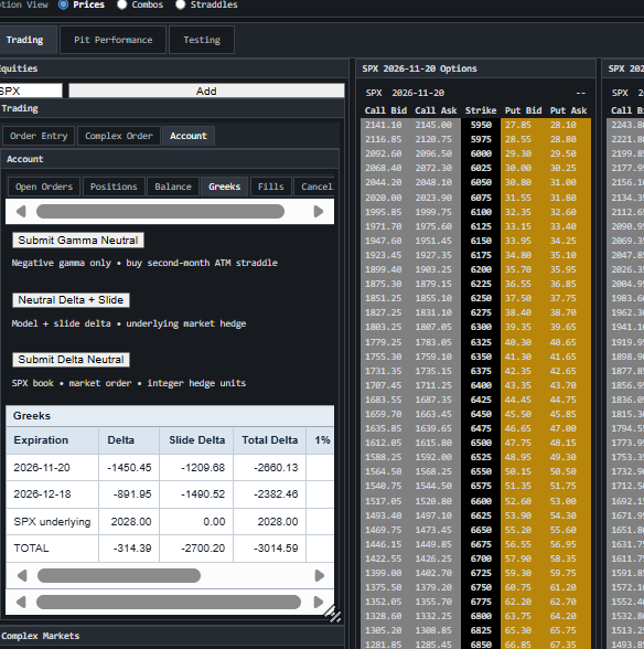
The gamma control addresses a short-gamma book by buying an at-the-money straddle in the second available expiration month at market. It sizes whole straddles to cover the estimated negative gamma, subject to execution and clearing approval.
Buying the straddle also changes delta, vega and time decay. That is part of the exercise. A trader who buys gamma during a falling market may reduce the need to keep selling the underlying into the decline, but the protection costs money.
You can reduce one risk and create another. The book has to be managed as a whole.
Watch the path, not just the finish
The pit screen plots each trader’s P&L alongside the spot path. A delta display helps explain whether a gain came with directional exposure, and settlement markers identify another point where the composition of the book can change.
The leaderboard separates realized and unrealized P&L and shows current Greeks and stress capital. A trade’s premium receipt is not automatically profit. Open positions must be valued, closed gains and losses must remain in the account, and the option multiplier must be applied consistently.
I am particularly interested in the variability of P&L changes. A trader who finishes ahead in one run may have taken a very different journey from a trader with a steadier book. Looking at both the result and the path makes this more informative than a simple arcade score.
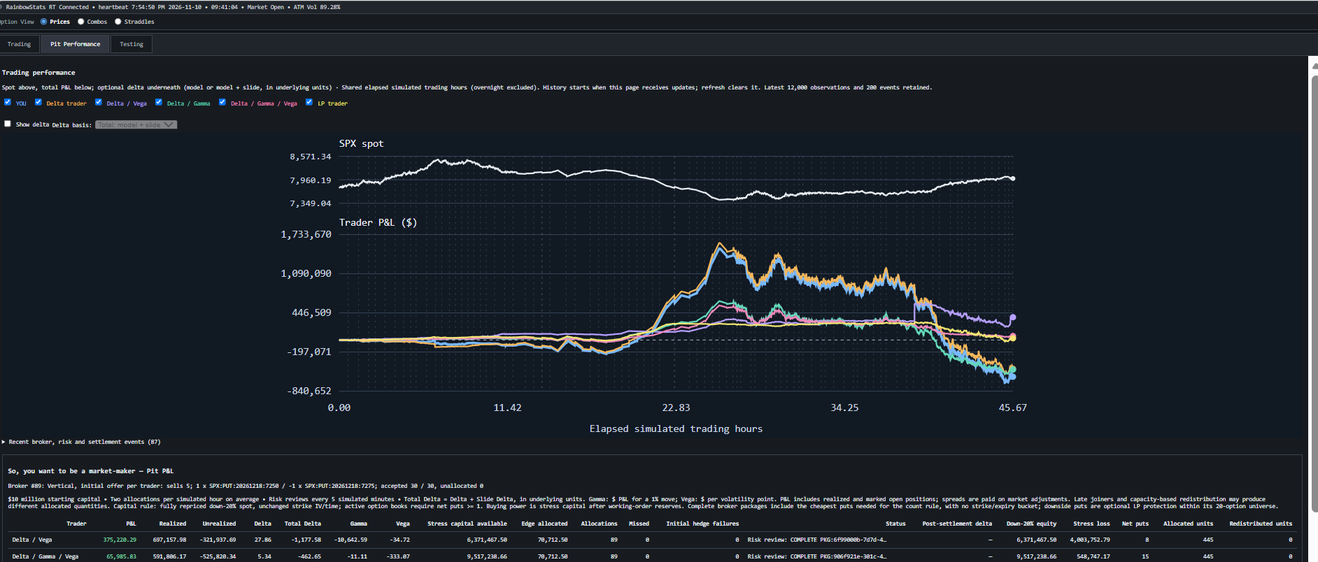
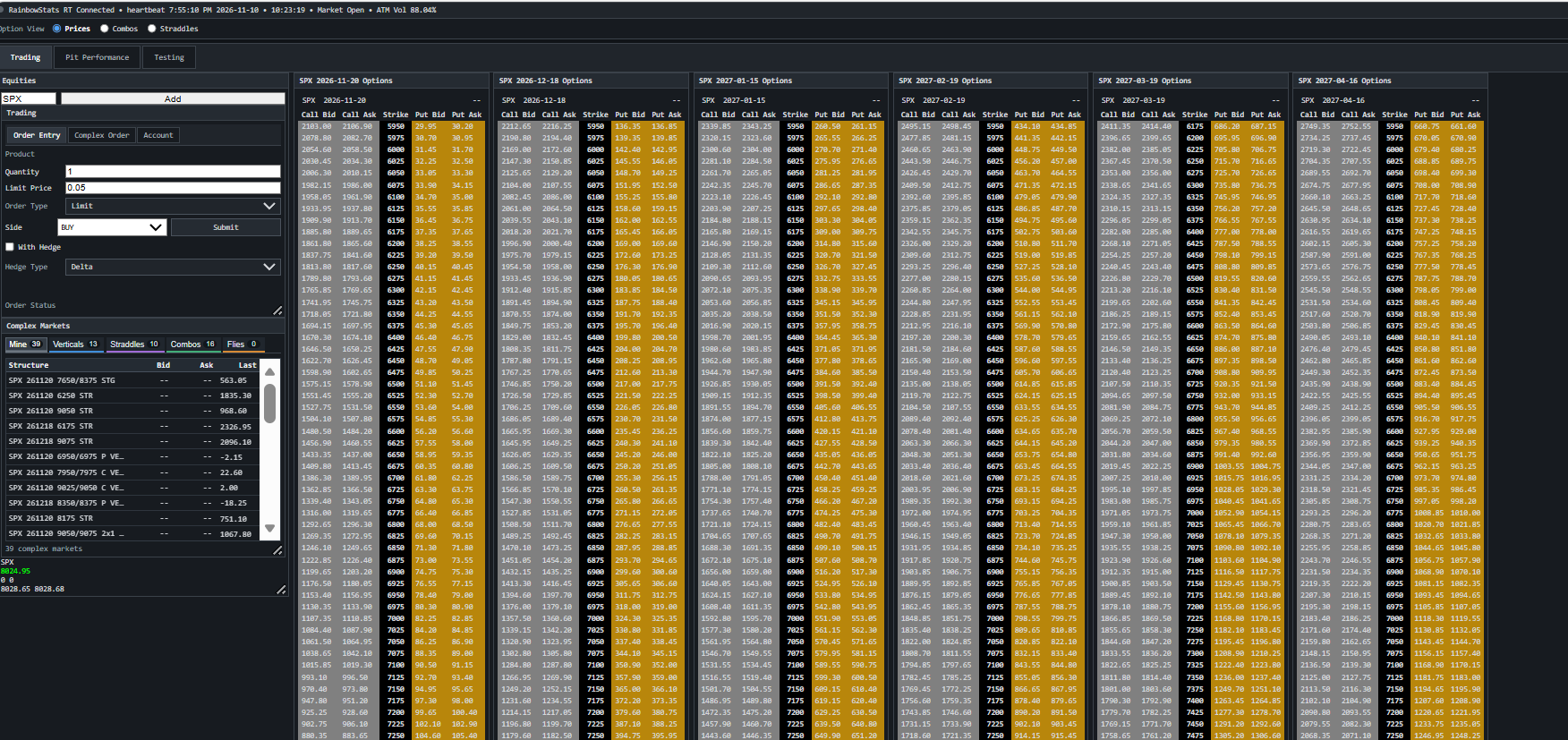
The screenshots were taken at different moments in a running simulation; their quotes, Greeks and P&L are not one synchronized portfolio snapshot.
Try keeping the edge
The original idea was a fun coding exercise. It has become a way to revisit a practical question from my years coding for traders in the pit: can you accept a steady flow of business, adjust the risk, pay for those adjustments, satisfy the clearing firm and still keep enough of the edge?
You can compete with the automated traders, experiment with the hedge controls, or simply watch how different books respond to the same market. A quiet session may flatter one strategy. A crash, a volatility change or an expiration can reveal something else.
The next research step is to run many reproducible scenarios and compare outcomes, trading costs and P&L variability. For now, there is a pit, a broker and a book to manage.
The next order is coming.
Try the market-making simulator →Notes on units, valuation and the model
Cash and contracts
Cash is measured in dollars. The simulator’s SPX option contracts use a multiplier of 100; the simulated underlying hedge uses a multiplier of 1. A quoted option premium of 10 therefore represents $1,000 per contract. This hedge instrument is a simulator convention.
Greek display units
Delta is shown in underlying-equivalent units after contract scaling. Vega is dollar P&L sensitivity per one volatility percentage point—for example, 20% to 21%. Gamma is displayed as the approximate second-order dollar P&L contribution for a 1% spot move. Those are different units; the numerical magnitudes should not be compared directly.
Local sensitivities and a large stress
Greeks describe local changes. The clearing test uses repriced instrument values at the stressed spot, rather than extrapolating a local delta or gamma over the entire 20% move. Actual replay outcomes can differ from that single stress assumption.
Faster calculations
The FFT wrapper checks native-library availability, numerical agreement and measured speed before selecting a backend. Production successfully selected FFTW. Java remains the fallback when native execution is unavailable or does not meet the selection criteria. Faster FFTs improve one part of pricing; networking, valuation and browser rendering still contribute to responsiveness.
Pricing references
- Madan, D. B., Carr, P. P., and Chang, E. C. (1998). The Variance Gamma Process and Option Pricing. European Finance Review, 2, 79–105.
- Carr, P., and Madan, D. B. (1999). Option valuation using the fast Fourier transform. Journal of Computational Finance, 2(4), 61–73.
This article describes a working simulator under development. The replay and risk rules are modeling choices for the exercise. All trading and account balances shown in the simulator are simulated.