A follow-up on place, mental distress and omitted variables
When Place Enters the Model
A reader asked whether the Washington–Iowa county comparison needed a state effect. Adding one does more than improve the fit: it changes the story the pooled regression was telling.
The links below open the earlier essay and the complete RainbowStats analysis with the state fixed effect.
Run the RainbowStats analysis Read the original blog
My daughter, a health care professional and one smart cookie, asked me to look at the state effect in my previous analysis, Fifty Years Later: The Human Toll of a Technological Society. It was exactly the right question: what happens if we control for the state in which each county sits?
The original model pooled Washington's 39 counties and Iowa's 99 counties into one cross-section. It related frequent mental distress to social isolation, food insecurity and county median income relative to the national median. The residual chart already hinted at the problem. The errors clustered by state: Washington counties often sat above the pooled prediction, while Iowa counties often sat below it.
That pattern is evidence that “place” contains information the pooled variables do not. A one-variable follow-up lets the two states have different baseline levels of reported distress. Iowa is the reference category, and a Washington dummy equals one for Washington counties and zero for Iowa counties.
The gain in explanatory power is not subtle
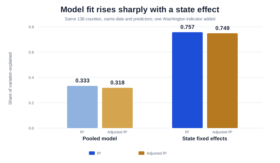
The pooled model explains 33.3 percent of the county variation in frequent mental distress. With the Washington indicator, R² rises to 75.7 percent. Adjusted R²—which penalizes the model for adding another variable—rises from 31.8 to 74.9 percent. The improvement is therefore not a cosmetic reward for adding a regressor.
The coefficients tell a different story
The state control does not merely absorb unexplained noise. It changes the estimated relationships among the original variables. Social isolation falls from 0.320 to 0.052 and is no longer statistically distinguishable from zero in this specification. Food insecurity remains positive, though its coefficient falls from 0.214 to 0.103. Relative income changes from essentially zero to a strong negative association.
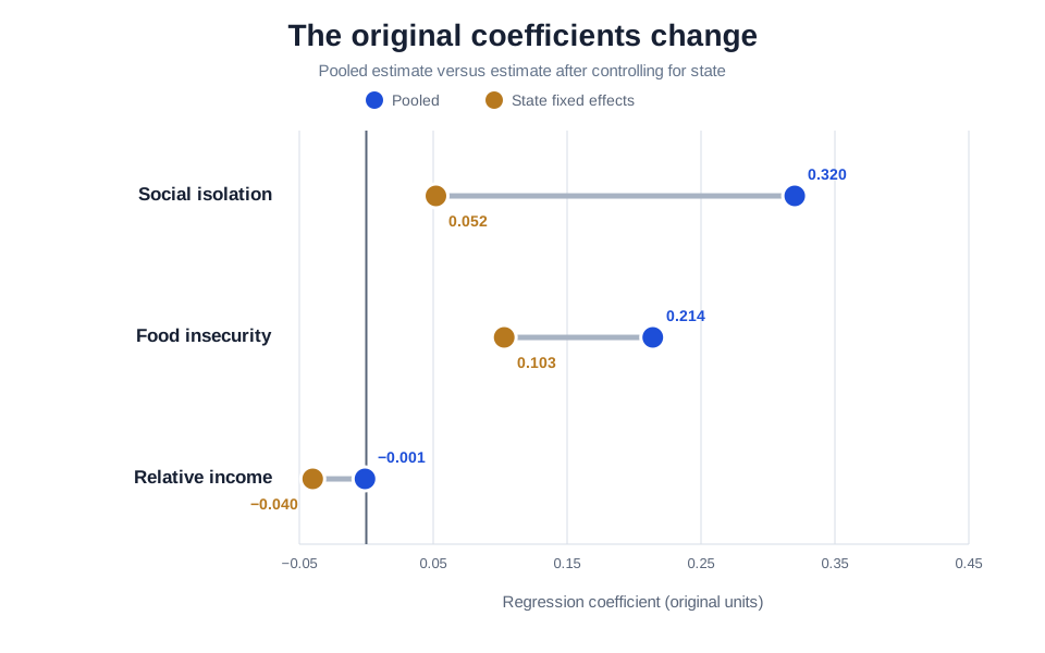
| Variable | Pooled β | Pooled t | State FE β | State FE t |
|---|---|---|---|---|
| Social isolation | 0.320 | 3.733 | 0.052 | 0.953 |
| Food insecurity | 0.214 | 3.691 | 0.103 | 2.882 |
| Median income relative to U.S. | −0.001 | −0.062 | −0.040 | −6.590 |
| Washington indicator | — | — | 2.624 | 15.218 |
A 2.6-point state gap
Conditional on the three measured county characteristics, the Washington indicator is 2.624 percentage points. In plain language, a Washington county is predicted to have about 2.6 percentage points more frequent mental distress than an Iowa county with the same measured isolation, food insecurity and relative income. Its conventional 95 percent confidence interval is approximately 2.29 to 2.96 points.
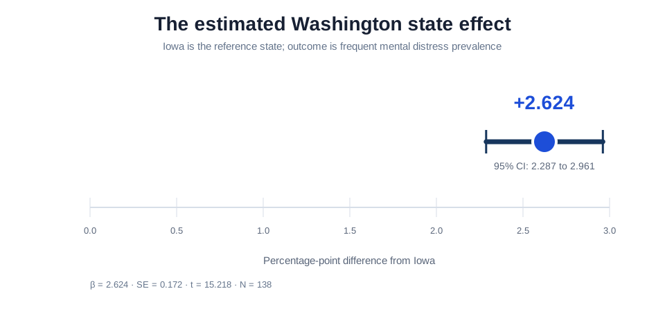
The magnitude explains why the pooled residuals separated by state. Without the indicator, the regression had to use isolation, food insecurity and income to approximate a baseline difference they could not fully represent. That is the omitted-variable problem in visible form: leave out a variable related to both the outcome and the included predictors, and the included coefficients may inherit part of its effect.
The outliers still matter
The state indicator removes the broad Washington–Iowa level difference, but it does not explain every county. The fixed-effects residuals now intermix the two states through most of the distribution. That is what we hoped to see: once the state baseline is controlled, the remaining errors are no longer separated into two obvious geographic camps.
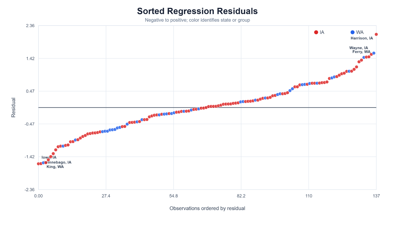
Yet the tails remain economically and substantively important. Harrison County, Iowa reports mental distress 2.108 percentage points above the model's prediction. Iowa County and Winnebago County, Iowa are about 1.62 points below prediction, while King County, Washington is 1.591 points below. On the positive side, Ferry County, Washington and Wayne County, Iowa are roughly 1.5 points above prediction.
These are not reasons to discard the model; they are invitations to investigate it. The state dummy captures a shared baseline, while the outliers point toward county-specific forces—local demographics, access to care, housing conditions, sampling variation or other omitted characteristics. A high R² can coexist with locally important exceptions.
The end of the road for the pooled hypothesis
In the earlier essay, we noted that a simple “end of the road” account was not enough to explain which individual Washington counties appeared in the residual tails. That remains true. The state indicator does not tell us why Washington differs from Iowa, nor does it identify a single Washington mechanism.
But it does mark the end of the road for the pooled model as a satisfactory explanation. Once state is controlled, the apparent independent association between isolation and distress largely disappears, income re-emerges, and food insecurity remains the more durable positive correlate. Most importantly, the state baseline dominates the comparison.
“State” is therefore a summary label, not an explanation. It may absorb differences in demographics, migration, housing burden, access to care, urban–rural composition, survey response, culture, institutions or variables not yet measured. The large R² tells us that geography matters; it does not tell us which part of geography is causal.
What we learned by adding one variable
The follow-up strengthens the central lesson of the original blog. Aggregate relationships can look persuasive while concealing the institutions and communities through which people experience economic and social conditions. The pooled result was not “wrong,” but it was incomplete. Its coefficients mixed variation within states with a substantial difference between states.
The responsible conclusion is modest. Across these 138 counties in 2022, food insecurity remains positively associated with frequent mental distress after allowing Washington and Iowa to have separate baselines. Relative income is negatively associated with distress within that controlled comparison. Social isolation, although important in the pooled model, no longer has an independently precise coefficient once state enters.
This is exactly why regression should be treated as an argument to be tested rather than a machine for producing final answers. A residual pattern raised a question. A state dummy answered part of it—and exposed the next question: what, specifically, does the state effect contain?
Sources, replication and cautions
- Complete RainbowStats replication with
STATE_FIXED_EFFECTS. - Fifty Years Later: The Human Toll of a Technological Society, the original analysis and interpretation.
- CDC PLACES county measures: frequent mental distress, social isolation and food insecurity.
- County and national median household-income series retrieved through FRED.
All results are exploratory and descriptive. They are based on aggregate county measures and conventional OLS standard errors. With only two states, state-clustered inference would not be reliable. The Washington coefficient should not be interpreted as a causal state effect, and county-level associations should not be transferred to individuals.