Money, Velocity, and Three-Stage Least Squares
A monthly monetary-system example using FRED data, a consumption-to-money velocity proxy, and Three-Stage Least Squares.
Most economic variables are not determined in isolation. Inflation affects interest rates, interest rates affect spending, and spending feeds back into inflation. That makes monetary analysis a natural setting for a simultaneous-equation model.
A common question is whether money creation itself causes inflation. The answer is not automatic. Money must be used in transactions before it can create pressure on consumer demand. Economists usually call this idea velocity.
The quantity of money, M, is only part of the equation. If velocity, V, falls because households save, businesses hold cash, or banks do not expand lending, then the effect on nominal spending may be muted. This is the old idea of pushing on a string: a central bank can make liquidity available, but it cannot force the private sector to spend or borrow.
Why Use a Monthly Velocity Proxy?
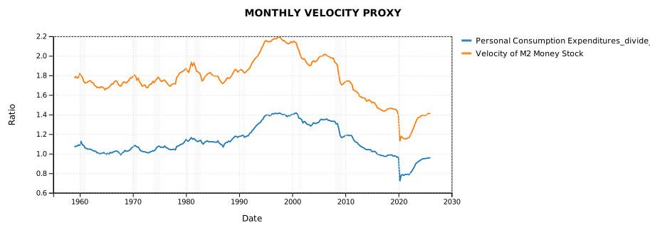
The official FRED series for M2 Velocity is quarterly. The other series in this example are monthly. To keep the system at a monthly frequency, I use a simple proxy:
This is not the official velocity measure, which is based on GDP divided by M2. Instead, it is a monthly consumption-to-money ratio. Since Personal Consumption Expenditures are the largest component of GDP, the proxy is a practical way to approximate how actively money is being used in the consumer economy.
Why should anyone care about velocity?
Imagine the Federal Reserve credits banks with an additional trillion dollars of reserves. If households increase savings and businesses postpone investment, much of that money remains idle. The money supply has increased, but consumer demand has not. Economists refer to this situation as "pushing on a string." Monetary policy can make funds available, but it cannot force people to borrow and spend. Inflation arises when money begins to circulate through the economy.
The RainbowStats Script
The full example can be run in RainbowStats here: Run the RainbowStats script.
VELOCITY = PCE / M2SL

set_title(
    Line_Chart(LIST(VELOCITY, M2V)),
    MONTHLY_VELOCITY_PROXY
)

r1 = REGRESSION(LOGDIFF(LIST(CPIAUCSL, PPIACO, VELOCITY)))

r2 = REGRESSION(LOGDIFF(LIST(PCE, CPIAUCSL, PAYEMS)))

r3 = REGRESSION(LOGDIFF(LIST(FEDFUNDS, CPIAUCSL, UNRATE, VELOCITY)))

s = SIMU_REGRESSION(r1, r2, r3)

t = THREE_STAGE_REGRESSION(
        s,
        LOGDIFF(LIST(PPIACO, PAYEMS, UNRATE, VELOCITY))
)

SLIDESHOW(t)
Series Used
| Code | Description | Role |
|---|---|---|
PCE |
Personal Consumption Expenditures | Consumer spending and numerator of monthly velocity proxy |
M2SL |
M2 Money Stock | Money stock and denominator of monthly velocity proxy |
CPIAUCSL |
Consumer Price Index for All Urban Consumers: All Items | Consumer inflation |
PPIACO |
Producer Price Index by Commodity: All Commodities | Producer price pressure |
PAYEMS |
All Employees, Total Nonfarm | Employment and real economy activity |
FEDFUNDS |
Federal Funds Effective Rate | Monetary policy rate |
UNRATE |
Unemployment Rate | Labor market slack |
M2V |
Velocity of M2 Money Stock | Quarterly benchmark for comparison |
The Three Equations
With the data synchronized to monthly observations, the example estimates three equations.
1. Inflation Equation
The first regression models monthly changes in consumer prices as a function of producer price inflation and the monthly consumption-to-money ratio.
CPI inflation = f(PPI inflation, monthly velocity proxy)Regression Results
| Name | Beta | Std.Error | T-Stat | Delta-R2 |
|---|---|---|---|---|
| Constant | 0.0025 | 0.0 | 28.002 | |
| Producer Price Index by Commodity: All Commodities_LogDiff | 0.205 | 0.0094 | 21.734 | 0.401 |
| Personal Consumption Expenditures_divide_M2_LogDiff | 0.027 | 0.0087 | 3.142 | 0.0065 |
| RSq | 0.41 | |||
| AdjRSq | 0.408 | |||
| DW Stat | 1.009 | |||
| SS Residuals | 0.0046 | |||
| Std Error | 0.0024 | |||
| AIC | -9,739.77 | |||
| BIC | -9,725.69 | |||
| F-Stat | 279.154 | |||
| Observations | 807 | |||
| Consumer Price Index for All Urban Consumers: All Items in U.S. City Average_LogDiff |
2. Consumption Equation
The second regression models monthly changes in consumer spending as a function of consumer prices and employment.
PCE growth = f(CPI inflation, payroll employment growth)Regression Results
| Name | Beta | Std.Error | T-Stat | Delta-R2 |
|---|---|---|---|---|
| Constant | 0.0028 | 0.0003 | 9.17 | |
| Consumer Price Index for All Urban Consumers: All Items in U.S. City Average_LogDiff | 0.43 | 0.071 | 6.086 | 0.065 |
| All Employees, Total Nonfarm_LogDiff | 0.884 | 0.038 | 23.316 | 0.377 |
| RSq | 0.443 | |||
| AdjRSq | 0.441 | |||
| DW Stat | 2.177 | |||
| SS Residuals | 0.031 | |||
| Std Error | 0.0062 | |||
| AIC | -8,211.08 | |||
| BIC | -8,197 | |||
| F-Stat | 320.233 | |||
| Observations | 807 | |||
| Personal Consumption Expenditures_LogDiff |
3. Policy Rate Equation
The third regression models monthly changes in the federal funds rate as a function of inflation, unemployment, and the velocity proxy.
Federal funds rate change = f(CPI inflation, unemployment, monthly velocity proxy)Regression Results
| Name | Beta | Std.Error | T-Stat | Delta-R2 |
|---|---|---|---|---|
| Constant | -0.017 | 0.0056 | -3.018 | |
| Consumer Price Index for All Urban Consumers: All Items in U.S. City Average_LogDiff | 5.853 | 1.323 | 4.425 | 0.053 |
| Unemployment Rate_LogDiff | -1.104 | 0.093 | -11.936 | 0.337 |
| Personal Consumption Expenditures_divide_M2_LogDiff | 4.842 | 0.515 | 9.4 | 0.06 |
| RSq | 0.452 | |||
| AdjRSq | 0.45 | |||
| DW Stat | 1.551 | |||
| SS Residuals | 10.174 | |||
| Std Error | 0.113 | |||
| AIC | -3,521.37 | |||
| BIC | -3,502.59 | |||
| F-Stat | 221.206 | |||
| Observations | 807 | |||
| Federal Funds Effective Rate_LogDiff |
Why Three-Stage Least Squares?
The three regressions are stored in the SIMU_REGRESSION operator. That object calculates the residual correlation and covariance matrix for the system. In other words, it asks whether the separate regressions contain hidden relationships in their residuals.
The THREE_STAGE_REGRESSION operator then takes the simultaneous regression system and an instrument list. It identifies endogenous right-hand-side variables, replaces them with fitted values from the first-stage regressions, and estimates the resulting system using the SUR/FGLS machinery.
Residual Correlation Matrix
| Code | Count | Mean | Std Dev | Consumer Price Index for All Urban Consumers: All Items in U.S. City Average_LogDiff_Residuals | Personal Consumption Expenditures_LogDiff_Residuals | Federal Funds Effective Rate_LogDiff_Residuals |
|---|---|---|---|---|---|---|
| Consumer Price Index for All Urban Consumers: All Items in U.S. City Average_LogDiff_Residuals | 807 | 0.0 | 0.0024 | 1 | 0.043 | 0.083 |
| Personal Consumption Expenditures_LogDiff_Residuals | 807 | 0.0 | 0.006 | 0.043 | 1 | -0.172 |
| Federal Funds Effective Rate_LogDiff_Residuals | 807 | 0.0 | 0.112 | 0.083 | -0.172 | 1 |
Three Stage Least Square Using SUR
| OLS Estimate | OLS Std Error (T-Stat) | SUR Estimate | SUR Std Error (T-Stat) | Std Error Improvement | Long Name | |
|---|---|---|---|---|---|---|
| Residual Dependence | ||||||
| Average residual corr. | 0.129 | |||||
| Average residual corr. | 0.254 | |||||
| Residual Dependence | Weak | |||||
| Efficiency | ||||||
| System OLS SSR | 10.206 | |||||
| System SUR SSR | 10.346 | |||||
| System SSR improvement | 0.987 | |||||
| Consumer Price Index for All Urban Consumers: All Items in U.S. City Average_LogDiff | OLS Estimate | OLS Std Error (T-Stat) | SUR Estimate | SUR Std Error (T-Stat) | Std Error Improvement | Consumer Price Index for All Urban Consumers: All Items in U.S. City Average |
| Constant | 0.0025 | 0.0 (28.025) | 0.0025 | 0.0 (27.95) | 1.001 | Constant |
| Producer Price Index by Commodity: All Commodities_LogDiff | 0.204 | 0.0094 (21.734) | 0.207 | 0.0094 (22.108) | 1.001 | Producer Price Index by Commodity: All Commodities |
| Personal Consumption Expenditures_divide_M2_LogDiff | 0.028 | 0.0087 (3.166) | 0.021 | 0.0087 (2.457) | 1.002 | Personal Consumption Expenditures_divide_M2 |
| OLS RSquare: | 0.41 | 0.41 | 0.41 | 0.41 | 0.41 | 0.41 |
| OLS DW: | 1.008 | 1.008 | 1.008 | 1.008 | 1.008 | 1.008 |
| Dates | 1959-02-01 | 2026-05-01 | 807 | |||
| Personal Consumption Expenditures_LogDiff | OLS Estimate | OLS Std Error (T-Stat) | SUR Estimate | SUR Std Error (T-Stat) | Std Error Improvement | Personal Consumption Expenditures |
| Constant | 0.0011 | 0.0004 (2.781) | 0.0011 | 0.0004 (2.83) | 1.001 | Constant |
| Consumer Price Index for All Urban Consumers: All Items in U.S. City Average_LogDiff_hat | 1.022 | 0.108 (9.487) | 1.01 | 0.108 (9.39) | 1.002 | Consumer Price Index for All Urban Consumers: All Items in U.S. City Average_hat |
| All Employees, Total Nonfarm_LogDiff | 0.834 | 0.037 (22.298) | 0.848 | 0.037 (22.804) | 1.006 | All Employees, Total Nonfarm |
| OLS RSquare: | 0.476 | 0.476 | 0.476 | 0.476 | 0.476 | 0.476 |
| OLS DW: | 2.163 | 2.163 | 2.163 | 2.163 | 2.163 | 2.163 |
| Dates | 1959-02-01 | 2026-05-01 | 807 | |||
| Federal Funds Effective Rate_LogDiff | OLS Estimate | OLS Std Error (T-Stat) | SUR Estimate | SUR Std Error (T-Stat) | Std Error Improvement | Federal Funds Effective Rate |
| Constant | -0.028 | 0.0077 (-3.706) | -0.019 | 0.0076 (-2.52) | 1.003 | Constant |
| Consumer Price Index for All Urban Consumers: All Items in U.S. City Average_LogDiff_hat | 9.586 | 2.156 (4.446) | 6.665 | 2.148 (3.103) | 1.004 | Consumer Price Index for All Urban Consumers: All Items in U.S. City Average_hat |
| Unemployment Rate_LogDiff | -1.126 | 0.093 (-12.107) | -0.963 | 0.092 (-10.525) | 1.016 | Unemployment Rate |
| Personal Consumption Expenditures_divide_M2_LogDiff | 4.477 | 0.541 (8.278) | 6.262 | 0.531 (11.784) | 1.018 | Personal Consumption Expenditures_divide_M2 |
| OLS RSquare: | 0.453 | 0.453 | 0.453 | 0.453 | 0.453 | 0.453 |
| OLS DW: | 1.566 | 1.566 | 1.566 | 1.566 | 1.566 | 1.566 |
| Dates | 1959-02-01 | 2026-05-01 | 807 |
What the Results Suggest
The strongest result is in the inflation equation. Producer prices are the dominant short-run driver of consumer prices. That is not surprising: changes in input and wholesale prices often pass through to consumer prices.
The velocity proxy is also positive and statistically significant, though its coefficient is much smaller than the producer price coefficient. This is the interesting monetary result. It suggests that the simple quantity of money is not the whole story. Money has to be spent, not merely created.
This explains why M2 growth alone can be a weak monthly predictor of inflation. During periods of uncertainty, households may save extra cash, businesses may postpone investment, and banks may hold reserves rather than expand credit. In that environment, central banks may be pushing on a string: liquidity is available, but private spending does not immediately follow.
Conclusion
This example does not claim that the PCE/M2 ratio is the official velocity of money. It is a monthly proxy for money utilization in the consumer economy. The proxy is useful because it behaves similarly to the official quarterly M2 velocity series while allowing monthly econometric analysis.
This study suggests that money creation alone is not enough to explain monthly inflation. Producer prices remain the dominant short-run driver of CPI, but a monthly consumption-to-money ratio adds statistically significant explanatory power. The results are consistent with the idea that money must circulate before it affects prices. Future work could compare this monthly proxy with other measures of spending intensity and investigate its performance during different monetary policy regimes.
The evidence points to a balanced conclusion: producer prices remain the primary short-run driver of monthly CPI inflation, but the consumption-to-money ratio adds information. Money creation alone is not enough. Inflation pressure rises when money circulates through spending.
Three-Stage Least Squares is a useful framework for this kind of question because inflation, spending, labor markets, and policy rates are not isolated variables. They form a system.