Using SUR Regression to Study Currency Exchange Rates
A practical RainbowStats example using domestic money velocity and U.S. money velocity
Seemingly Unrelated Regression, or SUR, is useful when several regression equations describe related markets. Each equation may have its own dependent variable and explanatory variables, but the unexplained shocks may be correlated across equations.
Currency markets are a natural example. The Canadian dollar, Brazilian real, Mexican peso, Japanese yen, and Australian dollar may each respond differently to local economic conditions, yet they are also exposed to common global and U.S. monetary shocks.
This example shows how RainbowStats can estimate the individual currency regressions, combine them into a
simultaneous system, and then apply the SUR_REGRESSION command.
The Economic Model
For each country, the regression relates the change in the exchange rate to the change in domestic money velocity and the change in U.S. money velocity. Recall in my previous blog I demmonstated how money velocity affects inflation.
Money velocity is calculated as:
The broad-money aggregate differs by country. The goal is not to force every country into a U.S.-style M2 definition, but to use a consistent broad monetary aggregate available for that country.
The RainbowStats Script
The full example can be run in RainbowStats here: Run the RainbowStats script.
GDP_US=GDP
GDP_BR=NGDPSAXDCBRQ
GDP_CA=NGDPSAXDCCAQ
GDP_MX=NGDPSAXDCMXQ
GDP_JP=NGDPSAXDCJPQ
GDP_AU=NGDPSAXDCAUQ

M2_US=MABMM301USM189S
M2_BR=MABMM301BRM189S
M2_CA=MABMM301CAM189S
M2_MX=MABMM301MXM189S
M2_JP=MABMM301JPM189S
M2_AU=MABMM301AUM189S

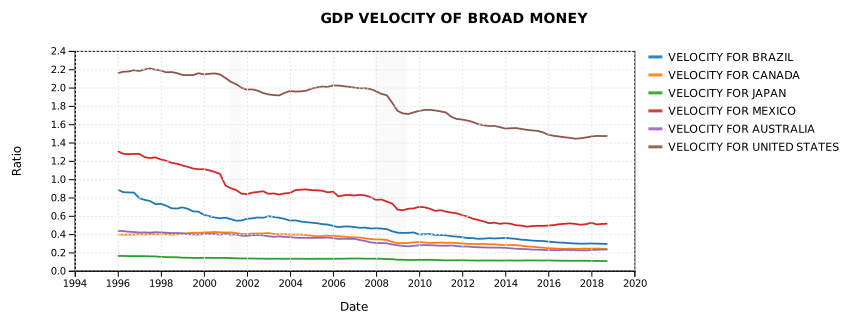
VEL_BR=Set_Name(GDP_BR/M2_BR,Velocity_for_Brazil)
VEL_CA=Set_Name(GDP_CA/M2_CA,Velocity_for_Canada)
VEL_MX=Set_Name(GDP_MX/M2_MX,Velocity_for_Mexico)
VEL_JP=Set_Name(GDP_JP/M2_JP,Velocity_for_Japan)
VEL_AU=Set_Name(GDP_AU/M2_AU,Velocity_for_Australia)
VEL_US=Set_Name(GDP_US/M2_US,Velocity_for_United_States)

line_Chart(
    same_date_range(
        VEL_BR,
        VEL_CA,
        VEL_JP,
        VEL_MX,
        VEL_AU,
        VEL_US
    )
)

CUR_BR=CCUSMA02BRQ618N
CUR_CA=CCUSMA02CAM618N
CUR_MX=CCUSMA02MXM618N
CUR_JP=CCUSMA02JPM618N
CUR_AU=CCUSMA02AUM618N

List_ALL=Same_Date_Range(
    List(
        CUR_CA,VEL_CA,
        CUR_BR,VEL_BR,
        CUR_MX,VEL_MX,
        CUR_JP,VEL_JP,
        CUR_AU,VEL_AU,
        VEL_US
    )
)

LIST_CA=list(
    ex(List_ALL,Series:0),
    ex(List_ALL,Series:1),
    ex(List_ALL,Series:10)
)

LIST_BR=list(
    ex(List_ALL,Series:2),
    ex(List_ALL,Series:3),
    ex(List_ALL,Series:10)
)

LIST_MX=list(
    ex(List_ALL,Series:4),
    ex(List_ALL,Series:5),
    ex(List_ALL,Series:10)
)

LIST_JP=list(
    ex(List_ALL,Series:6),
    ex(List_ALL,Series:7),
    ex(List_ALL,Series:10)
)

LIST_AU=list(
    ex(List_ALL,Series:8),
    ex(List_ALL,Series:9),
    ex(List_ALL,Series:10)
)

REG_CA=Regression(logdiff(LIST_CA))
REG_BR=Regression(logdiff(LIST_BR))
REG_MX=Regression(logdiff(LIST_MX))
REG_JP=Regression(logdiff(LIST_JP))
REG_AU=Regression(logdiff(LIST_AU))

Simu=SIMU_regression(
    REG_CA,
    REG_BR,
    REG_MX,
    REG_JP,
    REG_AU
)

sur=SUR_regression(Simu)
slideshow(sur)
Why the Script Calculates Velocity Before Applying LOGDIFF
The order of operations matters. The script first calculates the level of money velocity:
VEL_CA = GDP_CA / M2_CAIt then applies LOGDIFF to the complete regression list:
REG_CA = Regression(logdiff(LIST_CA))This produces the change in the logarithm of velocity:
That is the correct transformation. It measures the growth of nominal GDP relative to the growth of the money stock.
GDP / logdiff(M2) divides a level by a growth rate and is not a valid measure
of velocity.
An equivalent alternative would be to calculate GDP growth and money growth separately:
GDP_GROWTH = logdiff(GDP_CA)
MONEY_GROWTH = logdiff(M2_CA)
VELOCITY_CHANGE = GDP_GROWTH - MONEY_GROWTH
This is algebraically equivalent to applying LOGDIFF to the velocity ratio, apart from minor rounding
differences. The existing RainbowStats script is simpler and clearer.
Building the Individual Regressions
Each country is estimated separately first. In every list, the exchange rate is the dependent variable, domestic velocity is the first explanatory variable, and U.S. velocity is the second explanatory variable.
REG_CA=Regression(logdiff(LIST_CA))
REG_BR=Regression(logdiff(LIST_BR))
REG_MX=Regression(logdiff(LIST_MX))
REG_JP=Regression(logdiff(LIST_JP))
REG_AU=Regression(logdiff(LIST_AU))
Applying LOGDIFF transforms the exchange rates into approximate percentage changes and transforms
velocity into changes in monetary turnover. This is generally more appropriate than regressing exchange-rate
changes on trending levels.
Combining the Equations
The five regressions are combined into a simultaneous regression system:
Simu=SIMU_regression(
    REG_CA,
    REG_BR,
    REG_MX,
    REG_JP,
    REG_AU
)
The simultaneous system preserves the individual equations while allowing RainbowStats to compare their residuals and estimate the cross-equation covariance structure.
Applying SUR
The complete system is passed to the SUR estimator:
sur=SUR_regression(Simu)
slideshow(sur)
The output includes the OLS and SUR coefficients, standard errors, t-statistics, residual covariance and correlation matrices, system statistics, and efficiency comparisons.
Main Results
SUR Coefficient Comparison
| OLS Estimate | OLS Std Error (T-Stat) | SUR Estimate | SUR Std Error (T-Stat) | Std Error Improvement | Long Name | |
|---|---|---|---|---|---|---|
| Residual Dependence | ||||||
| Average residual corr. | 0.341 | |||||
| Average residual corr. | 0.699 | |||||
| Residual Dependence | Moderate | |||||
| Efficiency | ||||||
| System OLS SSR | 1.347 | |||||
| System SUR SSR | 1.357 | |||||
| System SSR improvement | 0.992 | |||||
| Currency Conversions: US Dollar Exchange Rate: Average of Daily Rates: National Currency: USD for Canada_LogDiff | OLS Estimate | OLS Std Error (T-Stat) | SUR Estimate | SUR Std Error (T-Stat) | Std Error Improvement | Currency Conversions: US Dollar Exchange Rate: Average of Daily Rates: National Currency: USD for Canada |
| Constant | -0.0093 | 0.0039 (-2.368) | -0.0079 | 0.0038 (-2.065) | 1.025 | Constant |
| VELOCITY FOR CANADA_LogDiff | -0.658 | 0.283 (-2.329) | -0.228 | 0.2 (-1.137) | 1.413 | VELOCITY FOR CANADA |
| VELOCITY FOR UNITED STATES_LogDiff | -1.19 | 0.388 (-3.065) | -1.445 | 0.366 (-3.947) | 1.061 | VELOCITY FOR UNITED STATES |
| OLS RSquare: | 0.226 | 0.226 | 0.226 | 0.226 | 0.226 | 0.226 |
| OLS DW: | 1.875 | 1.875 | 1.875 | 1.875 | 1.875 | 1.875 |
| Dates | 1996-03-31 | 2018-09-30 | 91 | |||
| Currency Conversions: US Dollar Exchange Rate: Average of Daily Rates: National Currency: USD for Brazil_LogDiff | OLS Estimate | OLS Std Error (T-Stat) | SUR Estimate | SUR Std Error (T-Stat) | Std Error Improvement | Currency Conversions: US Dollar Exchange Rate: Average of Daily Rates: National Currency: USD for Brazil |
| Constant | 0.0035 | 0.01 (0.336) | 0.0087 | 0.0099 (0.879) | 1.05 | Constant |
| VELOCITY FOR BRAZIL_LogDiff | -0.118 | 0.452 (-0.262) | 0.326 | 0.379 (0.86) | 1.193 | VELOCITY FOR BRAZIL |
| VELOCITY FOR UNITED STATES_LogDiff | -2.37 | 0.822 (-2.882) | -2.42 | 0.813 (-2.978) | 1.012 | VELOCITY FOR UNITED STATES |
| OLS RSquare: | 0.088 | 0.088 | 0.088 | 0.088 | 0.088 | 0.088 |
| OLS DW: | 1.544 | 1.544 | 1.544 | 1.544 | 1.544 | 1.544 |
| Dates | 1996-03-31 | 2018-09-30 | 91 | |||
| Currency Conversions: US Dollar Exchange Rate: Average of Daily Rates: National Currency: USD for Mexico_LogDiff | OLS Estimate | OLS Std Error (T-Stat) | SUR Estimate | SUR Std Error (T-Stat) | Std Error Improvement | Currency Conversions: US Dollar Exchange Rate: Average of Daily Rates: National Currency: USD for Mexico |
| Constant | 0.0051 | 0.0052 (0.985) | 0.0043 | 0.0051 (0.846) | 1.02 | Constant |
| VELOCITY FOR MEXICO_LogDiff | 0.257 | 0.218 (1.18) | 0.118 | 0.181 (0.656) | 1.207 | VELOCITY FOR MEXICO |
| VELOCITY FOR UNITED STATES_LogDiff | -1.856 | 0.516 (-3.598) | -1.711 | 0.495 (-3.456) | 1.042 | VELOCITY FOR UNITED STATES |
| OLS RSquare: | 0.13 | 0.13 | 0.13 | 0.13 | 0.13 | 0.13 |
| OLS DW: | 2.1 | 2.1 | 2.1 | 2.1 | 2.1 | 2.1 |
| Dates | 1996-03-31 | 2018-09-30 | 91 | |||
| Currency Conversions: US Dollar Exchange Rate: Average of Daily Rates: National Currency: USD for Japan_LogDiff | OLS Estimate | OLS Std Error (T-Stat) | SUR Estimate | SUR Std Error (T-Stat) | Std Error Improvement | Currency Conversions: US Dollar Exchange Rate: Average of Daily Rates: National Currency: USD for Japan |
| Constant | 0.0051 | 0.0061 (0.824) | 0.0039 | 0.006 (0.654) | 1.017 | Constant |
| VELOCITY FOR JAPAN_LogDiff | 0.807 | 0.568 (1.422) | 0.444 | 0.521 (0.852) | 1.09 | VELOCITY FOR JAPAN |
| VELOCITY FOR UNITED STATES_LogDiff | 0.147 | 0.578 (0.254) | 0.282 | 0.566 (0.497) | 1.021 | VELOCITY FOR UNITED STATES |
| OLS RSquare: | 0.03 | 0.03 | 0.03 | 0.03 | 0.03 | 0.03 |
| OLS DW: | 1.905 | 1.905 | 1.905 | 1.905 | 1.905 | 1.905 |
| Dates | 1996-03-31 | 2018-09-30 | 91 | |||
| Currency Conversions: US Dollar Exchange Rate: Average of Daily Rates: National Currency: USD for Australia_LogDiff | OLS Estimate | OLS Std Error (T-Stat) | SUR Estimate | SUR Std Error (T-Stat) | Std Error Improvement | Currency Conversions: US Dollar Exchange Rate: Average of Daily Rates: National Currency: USD for Australia |
| Constant | -0.011 | 0.0069 (-1.596) | -0.011 | 0.0066 (-1.676) | 1.039 | Constant |
| VELOCITY FOR AUSTRALIA_LogDiff | -0.622 | 0.449 (-1.386) | -0.647 | 0.309 (-2.09) | 1.45 | VELOCITY FOR AUSTRALIA |
| VELOCITY FOR UNITED STATES_LogDiff | -1.691 | 0.634 (-2.666) | -1.679 | 0.608 (-2.762) | 1.043 | VELOCITY FOR UNITED STATES |
| OLS RSquare: | 0.13 | 0.13 | 0.13 | 0.13 | 0.13 | 0.13 |
| OLS DW: | 1.759 | 1.759 | 1.759 | 1.759 | 1.759 | 1.759 |
| Dates | 1996-03-31 | 2018-09-30 | 91 |
Australia is the only country where domestic velocity also remains significant under SUR, with a t-statistic of approximately −2.1. Domestic velocity is weak or insignificant in the other equations, and Canada's domestic velocity loses significance after applying SUR.
| Finding | Interpretation |
|---|---|
| U.S. velocity is significant for Canada, Brazil, Mexico, and Australia | U.S. monetary conditions appear to be a common explanatory factor across several USD exchange rates. |
| Australia's domestic velocity is significant | Australia shows evidence that local monetary turnover contributes independently to currency movements. |
| Japan is insignificant | The Japanese yen does not follow the same pattern in this specification. |
| Equation R² values are modest | Velocity explains only a limited portion of exchange-rate variation, which is common in currency models. |
How to Interpret the SUR Gain
The residuals show moderate cross-equation correlation, which supports estimating the currencies as a related system. However, the practical gain from SUR is small.
The system sum of squared residuals is slightly worse, and the average efficiency improvement over OLS is limited. This does not mean SUR failed. SUR is designed to use cross-equation residual covariance to improve estimation efficiency. In this example, the correlations exist, but they are not large enough to materially change most of the coefficient estimates.
Statistical Cautions
- The equation R² values range from approximately 3% to 23%, so most exchange-rate variation remains unexplained.
- Durbin-Watson statistics below 2 in some equations suggest mild positive autocorrelation, which may make the reported t-statistics somewhat optimistic.
- Nominal GDP is quarterly while several broad-money and currency series are monthly. For a strict velocity calculation, monthly money stocks should ideally be converted to quarterly averages before division by quarterly GDP.
- Australia's historical broad-money series contains a major structural break. A later starting date, a break dummy, or removal of the affected observation may be appropriate.
- The regression identifies statistical association, not causation. U.S. velocity should be described as an explanatory factor rather than a proven driver.
Why This Is a Useful SUR Example
This script demonstrates the complete RainbowStats SUR workflow using real economic data:
- Download nominal GDP, broad money, and exchange-rate series.
- Calculate domestic and U.S. money velocity.
- Align all series to a common date range.
- Estimate each currency equation independently.
- Combine the regressions with
SIMU_REGRESSION. - Apply
SUR_REGRESSION. - Display the complete system with
SLIDESHOW.
Conclusion
Across five currency equations, U.S. money velocity is the only variable that consistently explains exchange-rate changes. Domestic velocity contributes independently only in Australia, while Japan shows no statistically significant relationship.
The modest SUR efficiency gains are also informative. They indicate that the currencies share some common shocks, but accounting for those correlations does not dramatically alter the individual regression results.
Most importantly, this example shows how a group of ordinary RainbowStats regressions can be converted into a simultaneous system with only two additional commands:
Simu=SIMU_regression(REG_CA,REG_BR,REG_MX,REG_JP,REG_AU)
sur=SUR_regression(Simu)
That makes SUR_REGRESSION practical for studying related markets, industries, countries, or economic
sectors whenever the individual equations may be connected through common residual shocks.
This example is intended as a demonstration of the RainbowStats workflow and not as investment advice.